Introduction
Each nation has its own program for performing calculations of the meteor phenomenon, with particular reference to dark flight. Such as the Spanish – Amalthea (J.M. Madiedo 2006), the Finnish – MC (Gritsevich, Maria et al. 2014), the Russian – Meteor Toolkit (Dmitriev, V. et al. 2018) or the Japanese – Fireball Inspector. (SonotaCo, 2010) I would like to introduce the program I wrote – MetLab – which is constantly being developed since 2015. The purpose of this article is not to present the operation of the program in detail, it merely provides a comprehensive picture of its current (2024) status. I do not plan to publish the program for the time being, it is only intended for personal use. It was also an essential tool for the calculations I published so far, and it will be more and more so in the future.
Beginnings
I started writing the program in 2015 using the Delphi programming language. At first, the goal was just to be able to convert between the many different coordinate formats with it. The information arrives in any format (Ra. – Dec.; Alt. – Az.; degrees/minutes – hours/minutes…etc.) I can calculate with them, these data must be saved / read back and can be converted with one click into the readable format for UFOOrbit. (SonotaCo, 2009) At that time, I began to deal more seriously with the calculation of the dark flight of fireballs, since there was no program available for this (not since then), neither free nor paid. In one year, I delved so much into the subject – among other things based on Ceplecha’s article (Ceplecha Z. 1987).- that I managed to program the first version of the dark flight calculation module in Delphi. Here I would like to point out that, as an amateur astronomer, I can only dedicate a small amount of my free time to meteoritics, which I have persistently did since the mid-90s. In 2020, I rewrote the entire program into C#, at which time I also rethought the user interface based on my experience so far. Many small new functions of the program have already been completed on the new interface, such as light curve display, dynamic mass calculation or the calculation and display of track parameters in 2D/3D.
The MetLab program
The program’s functions open separate windows, so it’s easy to customize exactly what you’re working with, and arrange it on the screen as you like.
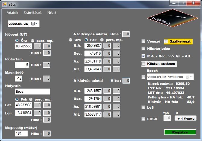
Figure 1 – Basic data window filled with one observation from Wien, 2022.06.24 a fireball above Austria
Basic data window – coordinate conversion
This is the main window (Figure 1) of the program, which opens first and the main data of the meteor fall can be entered, the conversion takes place, and the other functions can be accessed from here via the main menu. The time, duration, brightness of the fall, data on the location of the observation, the celestial coordinates of the start and the celestial coordinates of the end can be recorded. The program automatically handles and transforms if the data is entered with a dot or a comma-decimal separator. To accurately read the celestial coordinates, a crosshair can be activated, which remains active even outside the program window. The cursor can be moved pixel by pixel with the help of arrow keys and the environment of the reticle is displayed enlarged in a separate pop-up window, thus a pixel-accurate reading is available. By default, the coordinate calculations are made with the J2000 epoch, but this can also be changed. The calculated or uploaded data of the window can be transferred to other windows in one move, e.g. for the trajectory display to calculate the data of an intermediate section or for the trajectory calculation module (LoS) which is still under development. The basic and calculated data are changed dynamically if we prepare ECSV export step by frame for WMPL. (Vida, D. et al. 2019).
Functions available from the main menu:
Data:
– New data: Opens another basic data form window – in addition to keeping the original – if the main page is filled out, it automatically fills in the detection time data.
– Loading: loading previously saved data
– Save: save entered / calculated data
– R91 export: creating a file that can be read directly into UFOOrbit
– ECSV export: creating a file that can be read into WMPL
– Save / load location data: faster handling of detection location data
Calculations:
– Trajectory: opens the meteor trajectory data window
– Image analysis: you can work on the light curve of a meteor in this window
– Mass: opens the meteor fall mass calculation window
– Dark flight: the data of the dark flight of a meteorite fall can be entered in this window
– Line of Sight: trajectory calculation (under development) (Borovička J. 1990).
View:
– Enables switching between light and dark mode, which changes the colors of the user interface to colors that are easier on the eyes
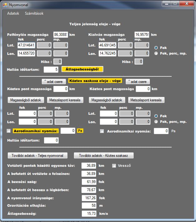
Figure 2 – Trajectory window filled with the data of 2022.06.24 fireball above Austria
Trajectory window
Here you can enter the data of the start and end point of the fall (Figure 2), the duration of the fall, from which the following parameters can be calculated:
– The length of the straight line between projection points
– Length of distance traveled on the surface
– Angle of incidence
– Distance traveled in the atmosphere
– Trajectory azimuth
– Gravitational deflection
– Average speed
At a specified height, it can calculate the coordinates of an intermediate point and the aerodynamic pressure (Bronshten, V.A. 1981) acting on the body there. The intermediate point can be recorded not only on the entered route, but also beyond it, e.g. thus a trail can be extended…
The program can search for the intersection of a detection entered in the Basic data window with the trajectory entered here.
All recorded or calculated data can be transferred to the dark flight calculation window with the press of a button.
The data can be saved in KML format: in 2D, it displays the surface projection in Google Earth, and in 3D, it represents the track in the atmosphere. (Figure 3)
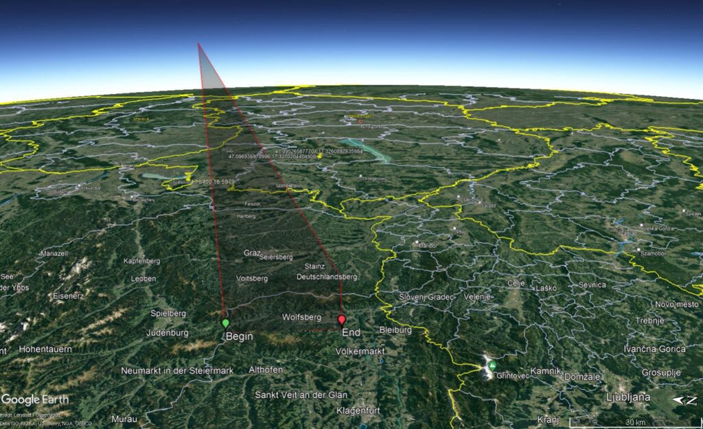
Figure 3 – 2022.06.24 Austrian fireball trajectory in 3D
Image analysis
The meteor photo can be processed in this window. By selecting the meteor in the image, the program creates a pixel database that can be read and converted under different conditions. The data read out pixel by row can be displayed in a light curve, at different points of which the height of the meteor can be displayed. The created light curve can be saved. The light curve can be calculated by subtracting the background lighting, highlighting the differences and stretching the axes to show each detail more accurately. (Figure 4)
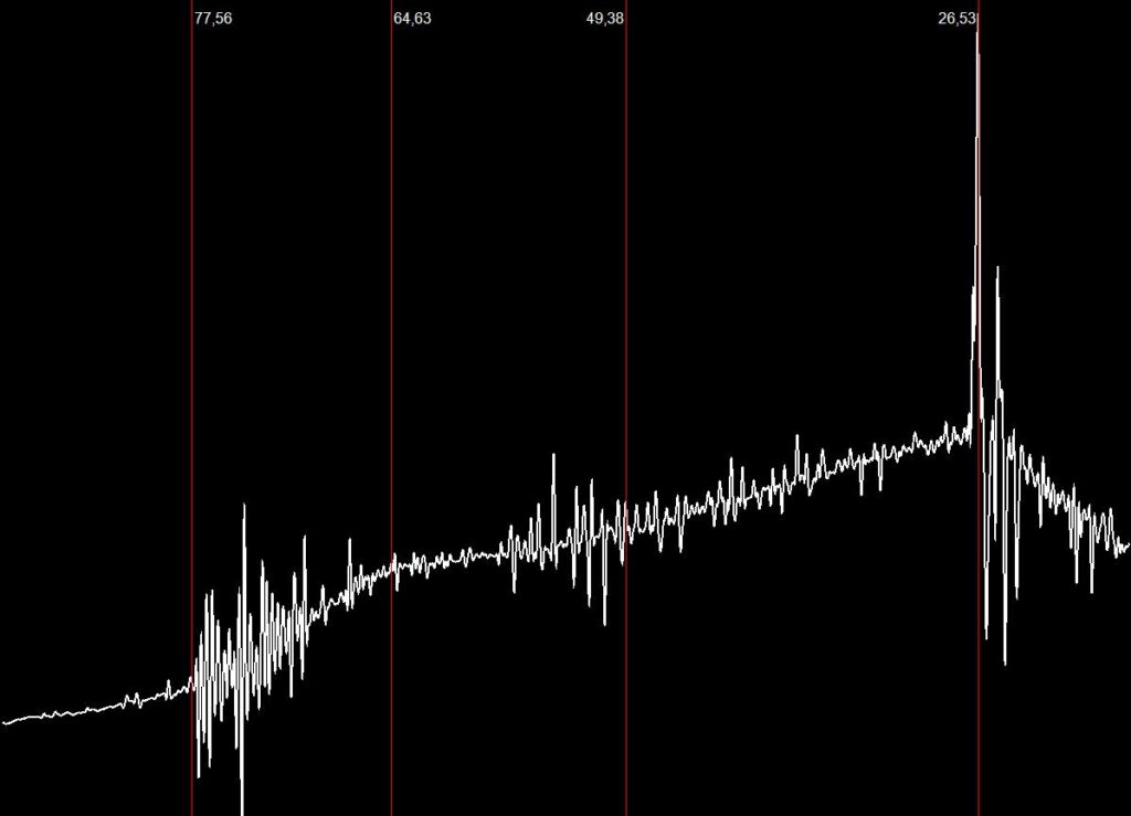
Figure 4 – The lightcurve of 2022.06.24 Austrian fireball, height is in ‘km’
Mass calculation
Based on the entered values, the mass of smaller meteors can be estimated by photographic mass calculation. (Jones et al., 1989) By entering the values read from the videos frame by frame, the dynamic mass of larger fireballs can be calculated. (Halliday et al. 1996) (Figure 5)
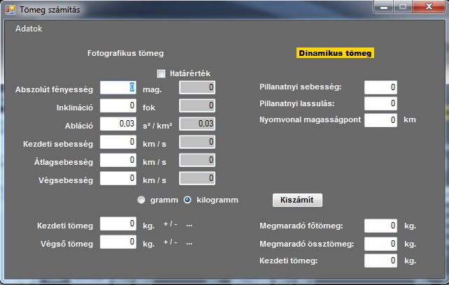
Figure 5 – The mass calculation window
Dark flight
By entering the parameters calculated at the end of the trajectory, the dark flight of the remaining mass can be modeled, further fragmentation is not yet calculated by the program. The stochastic simulation is performed using the Monte Carlo method with the specified limit values, in several thousand iteration steps down to the specified surface. It can start the pieces from a given point, a flat area, a given part of the space around the trajectory or a section of the trajectory. One of the most important parameter lists for performing the calculation is the upper atmospheric wind. The program can calculate from balloon wind measurements from one place or even interpolate the results of wind measurements from several places in space. Sounding data provided by University of Wyoming-Department of Atmospheric Science (http://weather.uwyo.edu/upperair/sounding.html) However, the most accurate results can be obtained with data from satellites refined with meteorological models. (GFS / NCEP / US National Weather Service) The program can calculate with all three methods at the same time, even with the weighting of these input data. The calculation result can be written out in CSV, in detail, for all the calculated data of each interpolation step in the case of 1 calculation. Also to CSV, only the data lines containing the final results, for each calculated piece. The most frequently used option is that the program saves the results in KML, which can be viewed immediately in Google Earth. The entire strewn field with all calculated data can also be exported to GPX, which can be loaded into a GPS to help on-site searches. (Figure 6 & 7)
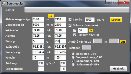
Figure 6 – The dark flight calculation window filled with the data of 2024.01.21 German fireball above Ribbeck
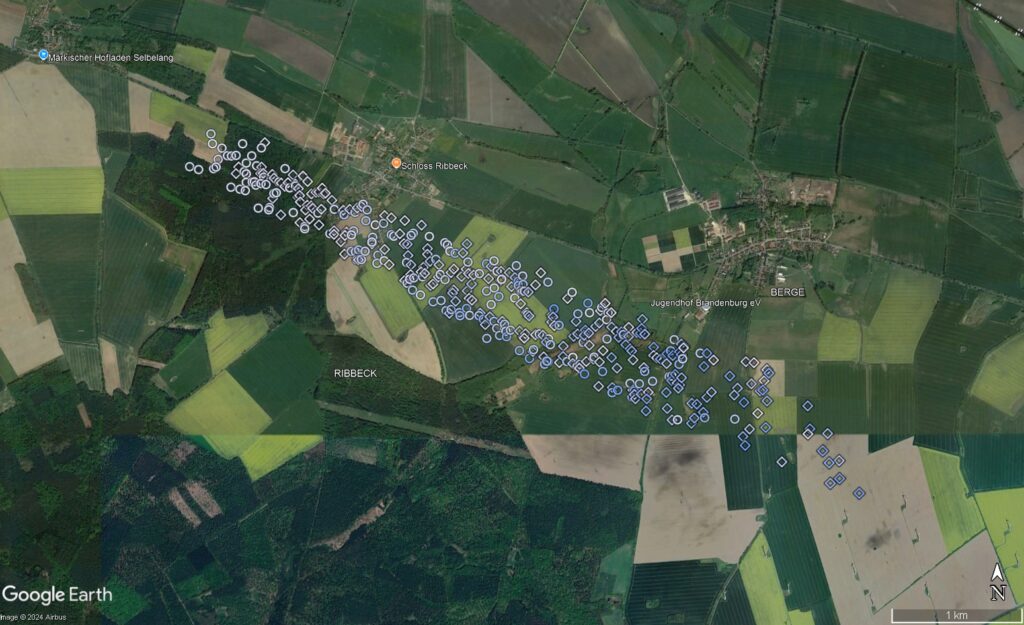
Figure 7 – The calculated strewn field with the initial data above. Blue – white ; higher or lower starting point, cube / circle resembles the shape of the meteorite
Vision – ongoing developments
The next important step is to program the trajectory calculation using the LoS method. This in itself would not be important, as there are programs available for free on the Internet. However, none of the programs deal with error propagation, which is essential for determining the standard deviation of the final results.
The graphical representation of the histogram and the RGB values read from the pixels will provide additional help for the analysis of the light curve. Another interesting thing could be the reading of a light curve using the current method, but from video material, frame by frame.
For a more complete picture of the strewn field, the simulation of further fragmentation during dark flight is also necessary.
I am constantly developing the program as I learn new formulas or more accurate data files.
References
J.M. Madiedo (2006). http://www.meteoroides.net/e_metobs_software.html
Gritsevich, Maria ; Lyytinen, Esko ; Moilanen, Jarmo ; Kohout, Tomáš ; Dmitriev, Vasily ; Lupovka, Valery ; Midtskogen, V. ; Kruglikov, Nikolai ; Ischenko, Alexei ; Yakovlev, Grigory ; Grokhovsky, Victor ; Haloda, Jakub ; Halodova, Patricie ; Peltoniemi, Jouni ; Aikkila, Asko ; Taavitsainen, Aki ; Lauanne, Jani ; Pekkola, Marko ; Kokko, Pekka ; Lahtinen, Panu ; Larionov, Mikhail (2014). “First meteorite recovery based on observations by the Finnish Fireball Network“. Proceedings of the International Meteor Conference, Giron, France, 18-21 September 2014 Eds.: Rault, J.-L.; Roggemans, P. International Meteor Organization, ISBN 978-2-87355-028-8, pp. 162-169
Dmitriev, V. ; Lupovka, V. ; Gritsevich, M. (2018). “Meteor Toolkit — Free Distributable Open-Source Software for Determination and Analysis of Meteoroid Orbits“. 81st Annual Meeting of the Meteoritical Society, held 22-27 July 2018 in Moscow, Russia. LPI Contribution No. 2067, 2018, id.6210
SonotaCo (2010). “meteor research processes Single Station Observation Measurement” https://slideplayer.com/slide/14945852/
SonotaCo (2009). “A meteor shower catalog based on video observations in 2007-2008”. WGN, Journal of the International Meteor Organization, 37, 55–62.
Ceplecha Z. (1987). “Geometric, dynamic, orbital and photometric data on meteoroids from photographic fireball networks”. Astronomical Institutes of Czechoslovakia, (Bulletin 38): 222–234.
Vida, D., Gural, P. S., Brown, P. G., Campbell-Brown, M., & Wiegert, P. (2019). “Estimating trajectories of meteors: an observational Monte Carlo approach–I. Theory“. Monthly Notices of the Royal Astronomical Society, 491(2), 2688-2705.
Borovička J. (1990). “The comparison of two methods of determining meteor trajectories from photographs“. Astronomical Institutes of Czechoslovakia, (Bulletin 41): 391
Bronshten, V.A. (1981). Geophysics and Astrophysics Monographs (Dordrecht: Reidel)
Jones J., McIntosh B. A. and Hawkes R. L. (1989). “The age of the Orionid meteoroid stream”. Monthly Notices of the Royal Astronomical Society, 238, 179–191.
Halliday, I., Griffin, A.A., Blackwell, A.T. (1996): “Detailed data for 259 fireballs from the Canadacamera network and inferences concerning the influx of large meteoroids“, Meteoritics & PlanetaryScience, 31, pp. 185 – 217
GFS / NCEP / US National Weather Service: https://www.ncei.noaa.gov/products/weather-climate-models/global-forecast
