The Earth-grazing Meteor of July 2024
Mark McIntyre
At 00:27:46 UT on the 7th of July 2024, an earth-grazer meteor was observed travelling from near Innsbruck in Austria to a point 30km north of Gravelines on the French coast. The meteor, travelling at 64km/s, traversed a distance of 841 km in 13.3 seconds at an altitude of between 114 and 102 km, crossing over Germany, Luxembourg, Belgium and France before returning to space. The event was detected by 35 cameras from the Global Meteor Network. A number of possible visual sightings were also reported to the IMO[1].
Analysis indicates that the meteoroid originated in the Kuiper Belt and likely last visited the inner solar system in 1536, the year in which Buenos Aires was founded and Anne Boleyn rose to and fell from power. In this article I present a summary of the results of manual data reduction and analysis. Full details of the event can be found on the UK Meteor Network’s website[2].
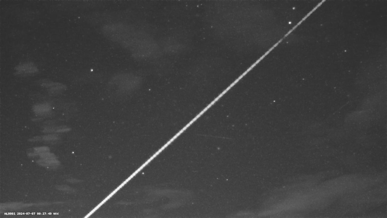
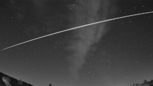
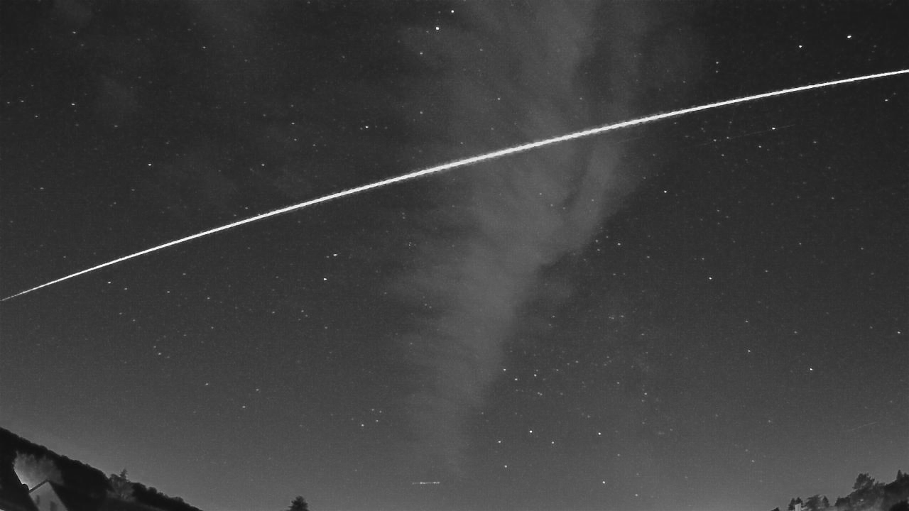
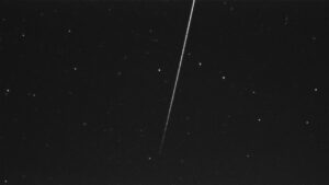
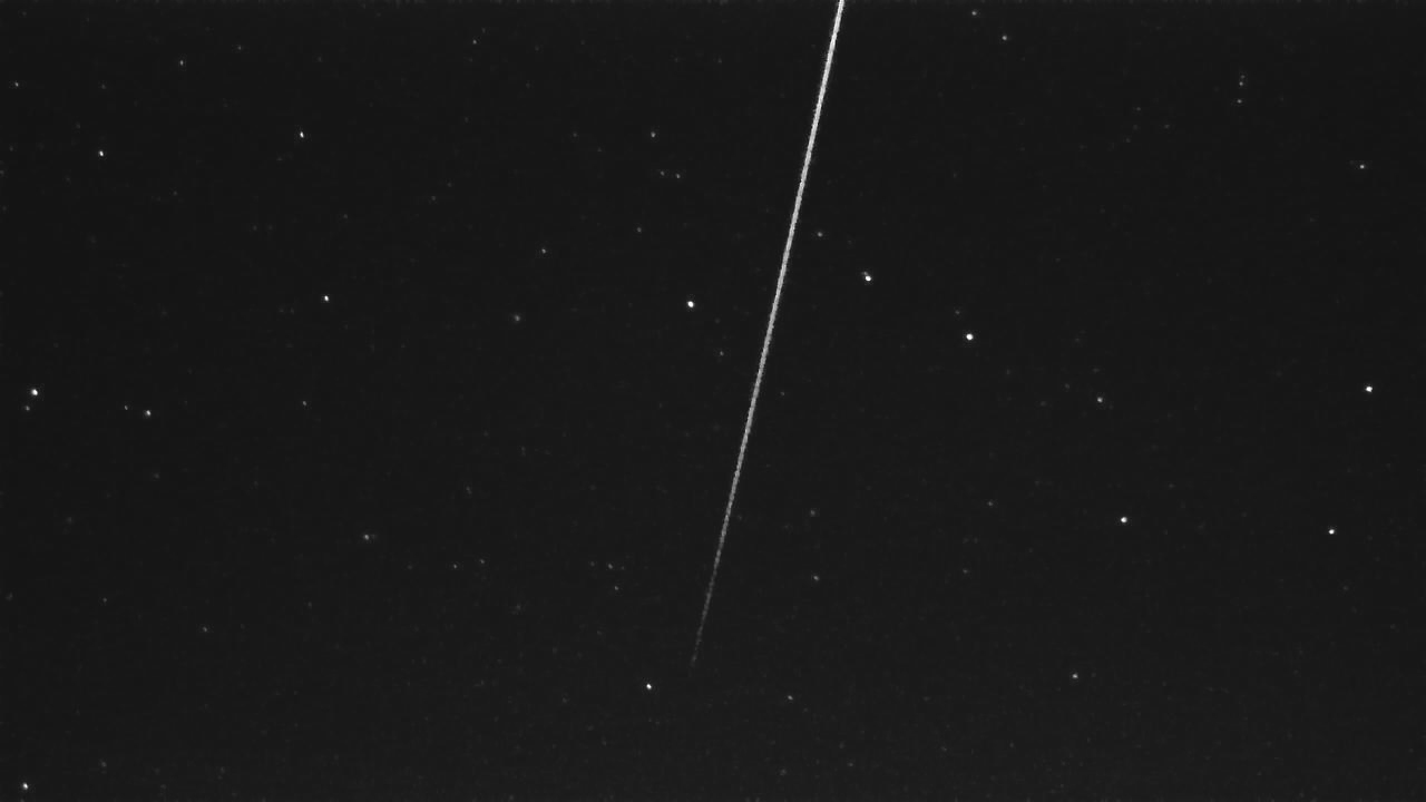
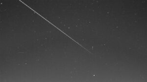
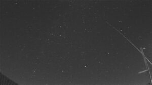
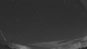
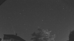
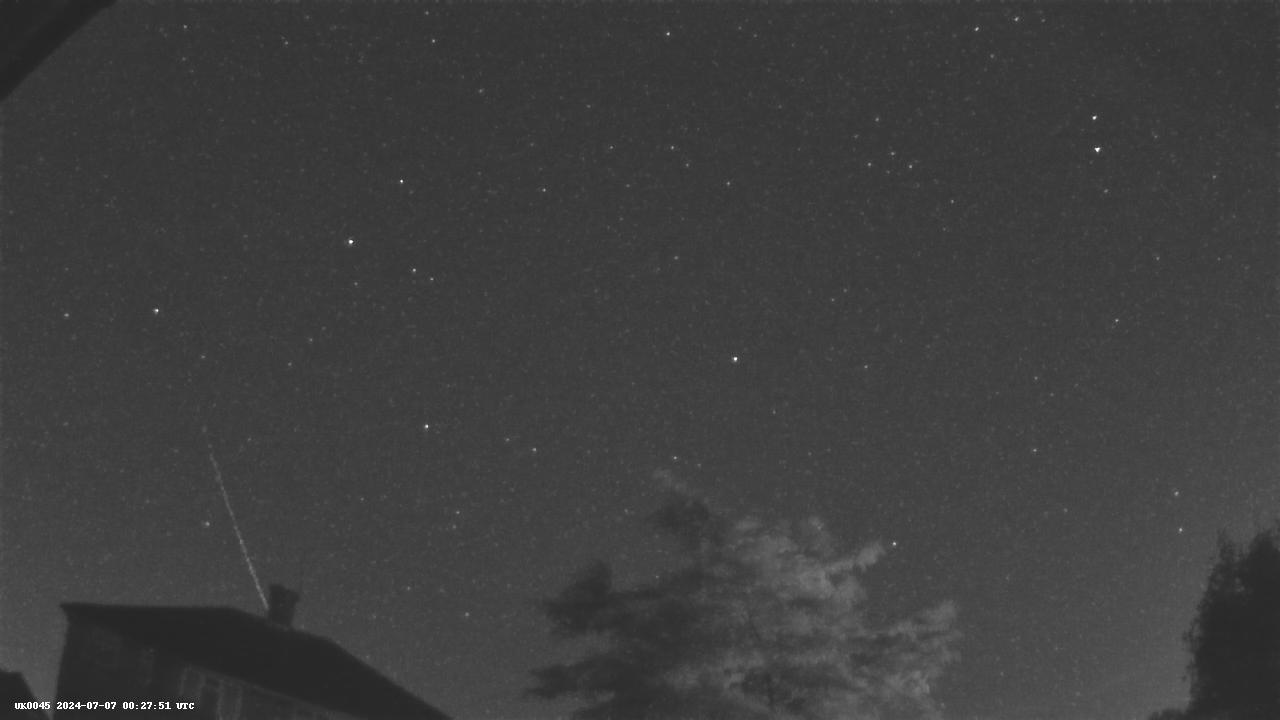
Figure 1: Meteor as seen from NL0001
1. Introduction
Earth-grazer meteors are meteors whose angle of entry into the atmosphere is so shallow that instead of penetrating downward, they skim across the surface and return to space. Earth-grazers are relatively rare as the likelihood of a meteor having a suitable entry angle of less than around +/- 2 degrees is low – see Gural, 2002[3].
As they usually present long tracks and are frequently observed over a very wide area visually and on camera they can look quite spectacular. However, due to considerable timing differences between observations, automated systems often misinterpret earth-grazers as multiple events on parallel tracks. To resolve such issues, manual analysis is required.
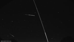
The event of 7th July 2024 was no exception. Picked up by cameras stretching from Croatia to England it was initially identified as two or possibly three parallel meteors.
2. Data Collection and Analysis
2.1 Collection
This event was detected by 35 separate cameras of the Global Meteor Network, GMN. GMN is a decentralised community of over 1000 cameras in 39 countries whose objective is to track and analyse meteors all around the world and which uses inexpensive security cameras optimised for low light detection, connected to a Raspberry Pi or Linux mini-PC running the opensource Raspberry Pi Meteor Station software, RMS. The methodology of data capture is further explained in Vida, et al., 2021[4].
Each camera generates a small payload containing an initial analysis of the detection, plus a video which can be further analysed. RMS has an Event Monitor facility which allows network coordinators to collect these data in near-real-time, and this was used to gather data from many cameras although multiple iterations were required as the meteor’s start and end points were initially unclear. Further data were also identified and collected by camera operators the following two days.
2.2 Selection and Analysis
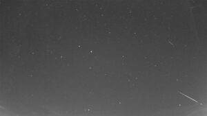
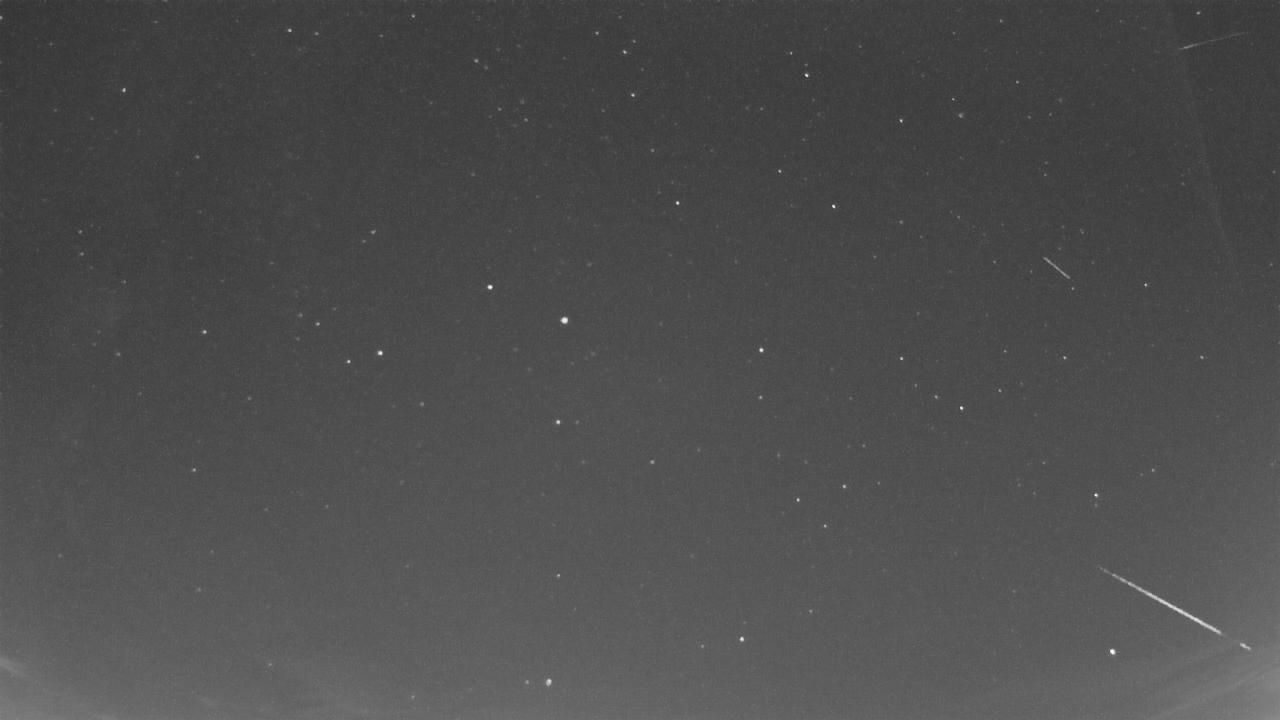
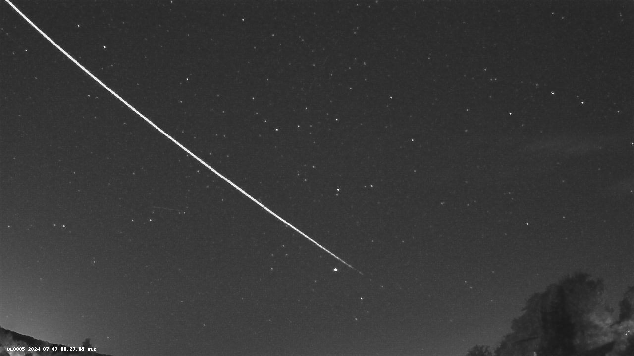
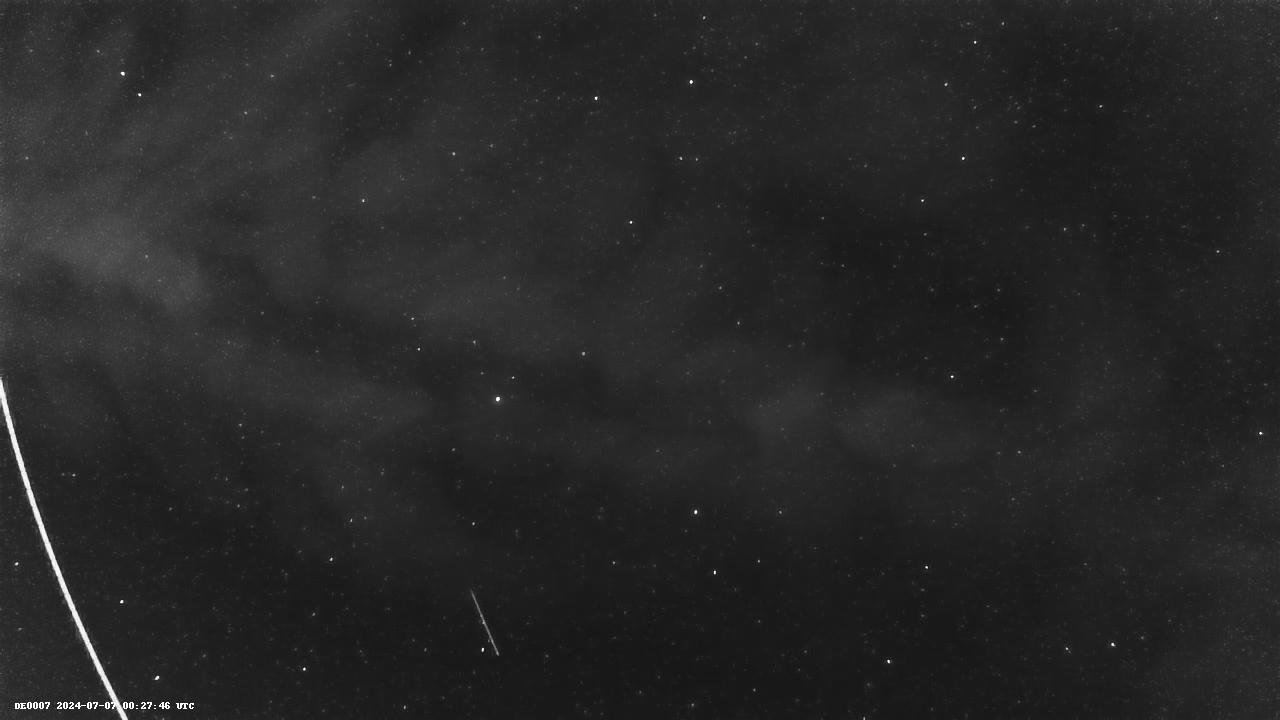
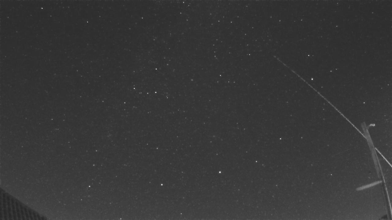
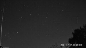
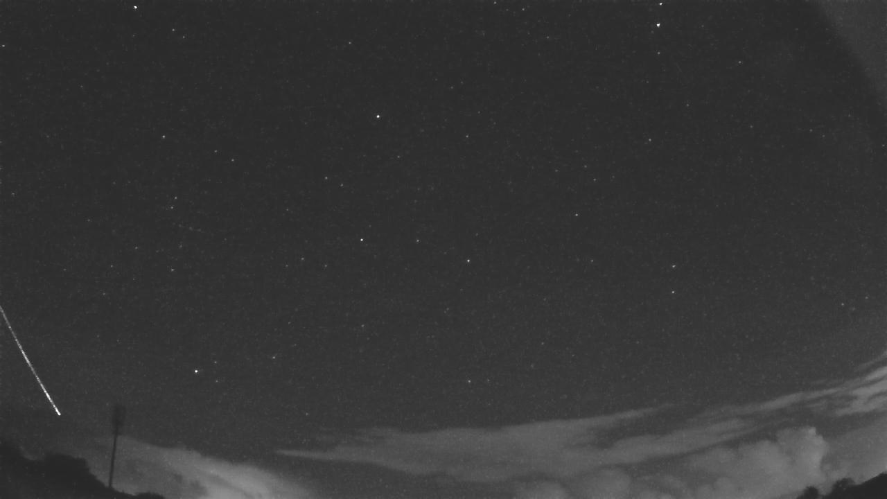
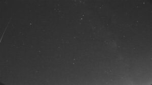
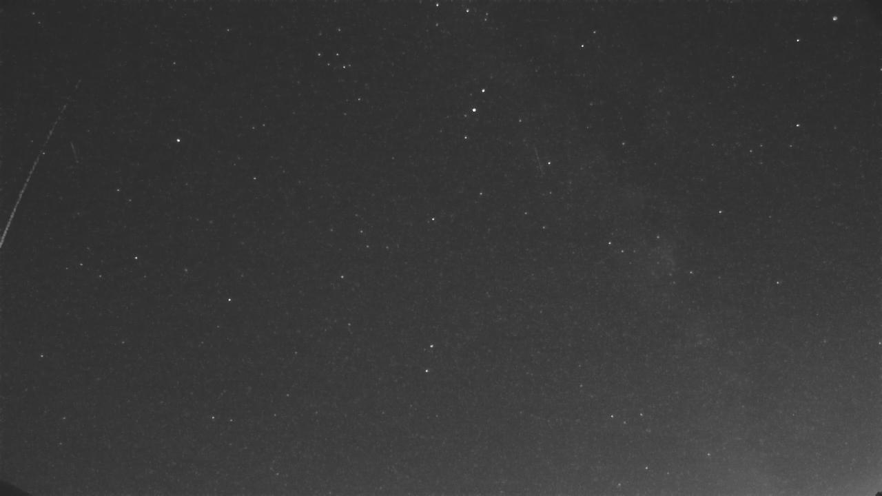
Although captured on numerous cameras, many contained only a partial view or were difficult to analyse due to obstructions in the field of view. Experience has shown that careful selection of good views can yield much better results, so fifteen cameras were chosen as providing the clearest or most useful views of the event. A full list of cameras is shown below, with cameras selected for analysis marked in bold. Stills from each of these cameras are shown below the table.
| BE000G | BE000J | BE000K | BE000V | BE0001 | BE0005 |
| BE0007 | BE0008 | DE0002 | DE0005 | DE0006 | DE0007 |
| FR000F | FR000G | FR000R | FR000X | FR000Y | FR0011 |
| HR000K | HR002R | NL000M | NL0001 | UK000F | UK00AF |
| UK00BC | UK00CJ | UK003W | UK0004 | UK004C | UK004E |
| UK006U | UK008C | UK009R | UK009X | UK0045 |
Table 1: Cameras
-
- HR002R
-

- DE0005
-
- DE0006
-

- DE0007
-
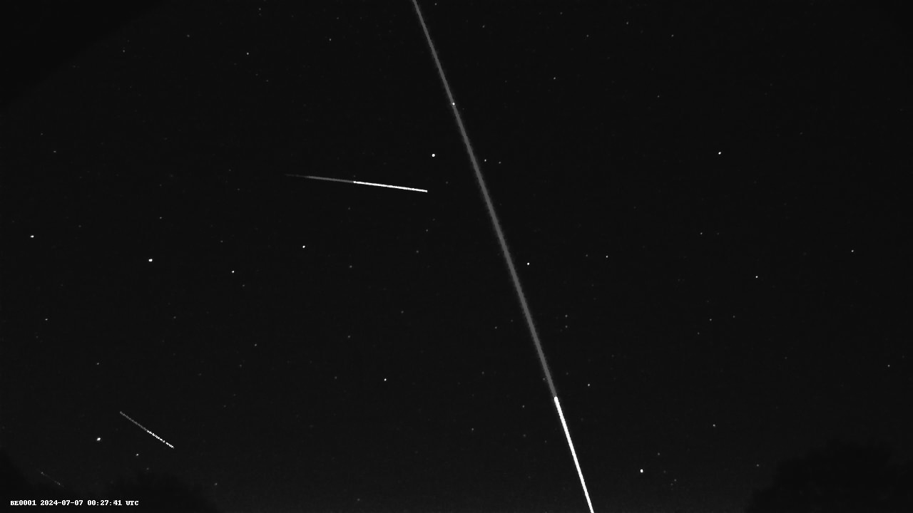
- BE0001
-
- BE0005
-

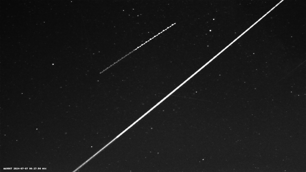
- BE0007
-
- BE0008
-
- FR000F

-
- FR000X

-
- UK00CJ
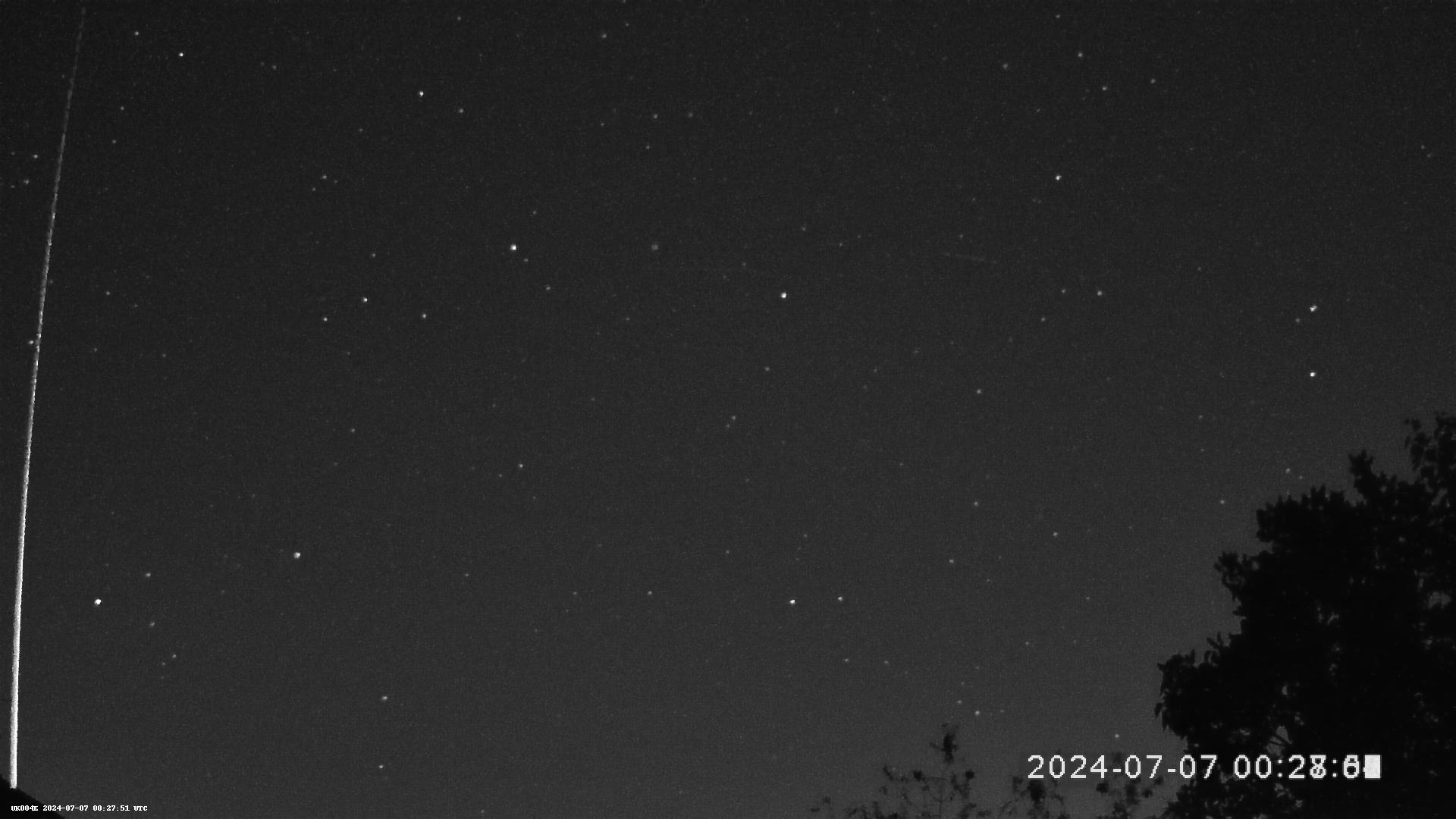
-
- UK004E
-
- UK008C
-
- UK009X
-
- UK0045
The video from each selected camera was then reanalysed. First, the field of view was recalibrated using the visible stars, geographic location of the camera and timestamp of the video. Next, the position of the meteor centroid was marked in each frame of video, allowing the brightness, bearing and angle of elevation of the detection to be determined on a frame-by-frame basis. There are further details in Vida et al (op cit).
2.3 Correlation
The data from the cameras were then correlated using the Western Meteor Python Library[5]. WMPL is a data analysis suite developed by the Western Meteor Physics Group at the University of Western Ontario. The tool performs an initial intersecting-planes solution on pairs of detections to determine if the pair admit of a physically realistic solution based on timestamp, fields of view overlaps, and so forth. Successful pairs are then merged into larger groups based on similar criteria. A Monte-Carlo model is then applied to each group to estimate a best fit trajectory to the data. The process is explained in more detail in Vida et al, 2019[6]
2.4 Initial failure
Initial attempts at correlation failed. Closer examination revealed that the correlator normally uses a ten second sliding window to decide whether cameras might be a matchable pair. However, in this case the duration of the event exceeded ten seconds and indeed some cameras had split the event into two videos. The ten-second sliding window was therefore insufficient to correlate between cameras with views of the start and end of the event, leading to overall failure.
To resolve this issue, the approximate duration was determined and the data were reanalysed with a wider sliding window of 15 seconds. This window is larger than the estimated duration and resulted in a successful solution.
3. Results
The object entered the atmosphere at an angle of attack of zero degrees, travelling at around 65.390 km/s +/- 0.004 km/s. It did not significantly decelerate during passage through the upper atmosphere. The duration of the event was calculated at 13.24 seconds from first detection over Austria to final detection over the English Channel.
It was not a bright event. Despite being widely detected, its best visual magnitude was only -1.4 and its best absolute magnitude -4.0. However, due to its longevity it looks quite spectacular on images and would have been very noticeable visually. Figure 1 is representative of the data collected by cameras. The GMN cameras have a field of view approximately 90 degrees by 45 degrees, so the visual size of this detection can be appreciated – to the human eye it would have appeared to traverse the entire sky in a few seconds.
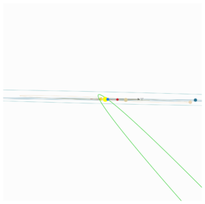
The tables below show details of the calculated trajectory and orbit. Figure 2 shows the location of the stations and the ground track of the meteor, while Figure 3 shows its computed orbit as seen from above the Sun’s north pole, and from a point in the plane of the ecliptic.
| Trajectory | Latitude (deg +N) |
95% CI (deg) |
Longitude (deg +E) |
95% CI (deg) |
Height MSL (m) |
95% CI (m) |
| Start Point | 47.1327 | 0.0001 | 11.9395 | 0.0002 | 117115 | 11 |
| Lowest | 49.3980 | 0.0000 | 6.9977 | 0.0000 | 102155 | 5 |
| End Point | 51.2928 | 0.0001 | 2.1426 | 0.0002 | 114929 | 10 |
Table 2: Ground Track and Altitude
| Orbital Characteristics | Value | 95% CI |
| Orbital Period T | 488 years | 15 years |
| Semimajor axis a | 62.01 AU | 1.25 AU |
| Eccentricity e | 0.98817 | 0.0002 |
| Inclination i | 139.956 | 0.003 |
| Solar Longitude | 105.066319 | 0.000002 |
| Last Perihelion | 1536 CE |
Table 3: Pre-atmospheric Orbital Characteristics
-
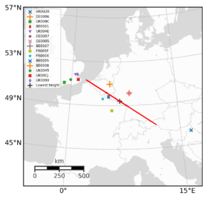
- Figure 2: Ground Track and Stations
-
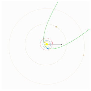
- Figure 3a: Top view of Orbit
-
- Figure 3b: Side view of Orbit
Further analysis and data, including additional still photographs and some short video clips are available on the UK Meteor Network’s website[7].
4. Discussion
4.1 Difficult Analysis
Despite being detected by many cameras, this event was surprisingly hard to analyse, requiring several days of effort. There were a number of reasons for this.
Firstly, to collect in near-realtime it is necessary to have an estimate of the start and end points so that RMS can determine which cameras should have a view. However in this case, initial estimates of the start were inaccurate by several degrees, as the detection by the camera in Croatia was not initially spotted. This led to some other cameras being initially overlooked.
Secondly, RMS collects data in ten second blocks, and as this event spanned more than ten seconds, several cameras split the event over two blocks. This complicated analysis as due to the time taken to reset the camera, there is always a small gap between videos. Consequently, care had to be taken during the recalibration and analysis of individual videos.
Furthermore, as mentioned earlier, the normal ten second sliding window proved inadequate and a larger window of fifteen seconds had to be used. A lesson to be learned from this is that when analysing long-duration events, the sliding window must always be large enough to encompass both start and end points.
4.2 Trajectory
As shown in Table 2, the trajectory of this event curved downwards and then back up. However, this is not quite correct! As Figure 4 shows, the trajectory was in fact very near to a straight line. The apparent track curvature is due to the curvature of the Earth itself. Studies of previous earth-grazers have often shown a similar effect.
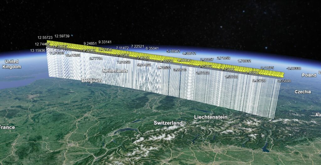
Figure 4 Google Earth 3d representation of trajectory
4.3 Orbit and Origin
The calculated orbit indicates that the object originated in the Kuiper belt. Normally, some degree of caution is required with orbits that seem highly eccentric as quite often, this is an artefact of high levels of uncertainty in the results due for example to poor viewing angles from one of the cameras. However, in this case the uncertainties in the data are low and so perhaps we can infer the origin with more confidence.
5 Conclusion
This was an interesting if difficult object to analyse, and some important lessons were learned which will aid with future analysis. In particular, quicker and more accurate estimation of the start and end points and of the duration is important.
It’s unfortunate that this object wasn’t larger and didn’t arrive at a different angle of attack. If that had been the case, there’s a possibility it might have dropped meteorites of Kuiper Belt origin which would have been very interesting to study.
6 Acknowledgements
I’d like to thank Steve Wyn-Harris who first brought this event to our attention and Jamie Shepherd, Milan Kalina, David Rollinson, Jorgen Dorr, Paul Roggemans, Jamie Olver, Nick James and Denis Vida who helped with obtaining and analysing data. I’d also like to thank the camera operators whose cameras detected the event, and all other operators whose cameras have helped in the past and will help again in the future.
Mark McIntyre, Tackley Observatory, Oxfordshire, UK.
7. References
[1] https://ukmon.imo.net/members/imo_view/event/2024/3306
[2] https://archive.ukmeteors.co.uk/reports/2024/orbits/202407/20240707/20240707_002746.047_UK/index.html
[3] Gural, P. S. (2019). On the frequency of pointer meteors and grazers. WGN, Journal of the International Meteor Organization, vol. 30, no. 5, p. 149-151
[4] Vida, D., Segon, D., Gural, P.S., Brown, P.G., McIntyre, M.J., Dijkema, T.J., Pavletic, L., Kukic, P., Mazur, M.J., Eschman, P. and Roggemans, P., (2021). The Global Meteor Network – Methodology and first results. Monthly Notices of the Royal Astronomical Society, 506(4), pp.5046-5074
[5] See https://github.com/wmpg/WesternMeteorPyLib/tree/master
[6] Vida, D., Gural, P. S., Brown, P. G., Campbell-Brown, M., & Wiegert, P. (2019). Estimating trajectories of meteors: an observational Monte Carlo approach–I. Theory. Monthly Notices of the Royal Astronomical Society, 491(2), 2688-2705.
[7] https://archive.ukmeteors.co.uk/reports/2024/orbits/202407/20240707/20240707_002746.047_UK/index.html
