by David Holman, Peter Jenniskens
Abstract: Radiant maps that display meteor direction and speed at a given time in the year also map the orbital elements of the meteoroid. Here, we present a number of all-sky radiant maps from six full years of CAMS meteor video observations that are color coded by meteoroid orbital element. The plots show that some orbital elements have a very organized distribution of values across the sky resulting in well-defined color zones, as these are mostly determined by the radiant position, while the elements that are determined mostly by speed tend to show a mixed distribution of values and colors. Because both Apex and Anthelion sources have mostly a limited range in speed, the use of D criteria does not always easily define a shower among the nearby sporadic background.
1 Introduction
When viewing meteor radiant maps like those in Jenniskens (2023), or those shown on the CAMS website, it is rarely appreciated how the location of a radiant on the sky is diagnostic of the orbit of the meteoroid. That is because the maps are for a limited period of time in the year and the range of speed is fairly limited for meteors arriving from a given direction.
The time, direction and speed at which a meteoroid enters Earth’s atmosphere are typically expressed as solar longitude (which determines the position of Earth around the Sun), the Right Ascension and Declination of the radiant, and the Speed. From that, the six Keplerian orbital elements of a meteoroid are calculated: the perihelion distance q (AU), semi-major axis a (AU), eccentricity e, inclination i (°), argument of perihelion ω (°), and node Ω (°), where a, e and q are related according to q = a (1 – e).
Derivative parameters include the Öpik parameters U, ϕ (°), and cosine θ, the longitude of perihelion Π (°) = ω + Ω, and the Tisserand parameter with respect to Jupiter TJ.
Others have plotted full annual activity in equal area plots, usually mapped with a vg color scale. Examples include the back covers of WGN by Molau and Rendtel (2009) and SonotaCo (2009). Also plots by Koukal (2016) and Koukal et al., (2024) which appeared in eMetN.
Here, we will show how to read radiant maps by showing how the orbital elements change for different directions in the sky over the course of the full year. We will show a series of all-sky plots of radiants in Sun-centered ecliptic longitude and ecliptic latitude, with orbital element values color coded.
2 Methods
The maps display the data in the CAMS Meteoroid Orbit Database v3.0 (Jenniskens et al., 2018). The database runs until the end of 2016, while much more data was taken in recent years that cover the southern hemisphere better. However, every single triangulation in this earlier data set was manually verified.
The maps were created using a newly developed MATLAB script which makes all-sky, all-year plots with nearly equal x and y axis scales in a cylindrical projection. The plot axes are in Sun-centered ecliptic longitude (“longitude”) and ecliptic latitude (“latitude”). Each radiant marker is plotted in a color corresponding to the element value of that radiant, and the element values are mapped to the MATLAB ‘turbo’ color map.
A second MATLAB script creates an interactive version of each plot that was used to check for obscured data in dense clusters, determine local means and variance, and to identify the elements of radiants that appear “out of zone”, i.e., a different color than the background. While the plots show a full year of activity at once, each element was examined with plots of a 20° solar longitude period that were advanced 5° at a time producing a 72 frame “movie” to check for possible zone changes during the year.
3 Keplerian element distributions
Figures 1–11 show these orbital element distributions.
The CAMS low-light video observations show the main source directions: the northern and southern halves of the Apex, the Antapex, the Anthelion, and the Toroidal ring.
The Helion, southeastern quadrant of the Apex, and southern and western Antapex are not as well observed because the dataset is based on observations to the end of 2016 and does not include results from the southern hemisphere expansion in recent years. The corresponding maps of more recent video data, and radar data, are shown in Jenniskens (2023, p.128 and p.130, respectively).
Other interesting features include a void of radiants in the Apex source near the ecliptic plane. The lack of data in this region is not an observational artifact, but due to a real lack of meteoroid orbits in the ecliptic plane from planetary perturbations.
There is also a lack of radiants between the Apex source and Toroidal sources, in a region surrounding the Apex source. Here, this empty region will be referred to as the “transition region”, split as the eastern and western transition regions. The western transition region is well observed by CAMS while the eastern transition region suffers from daylight.
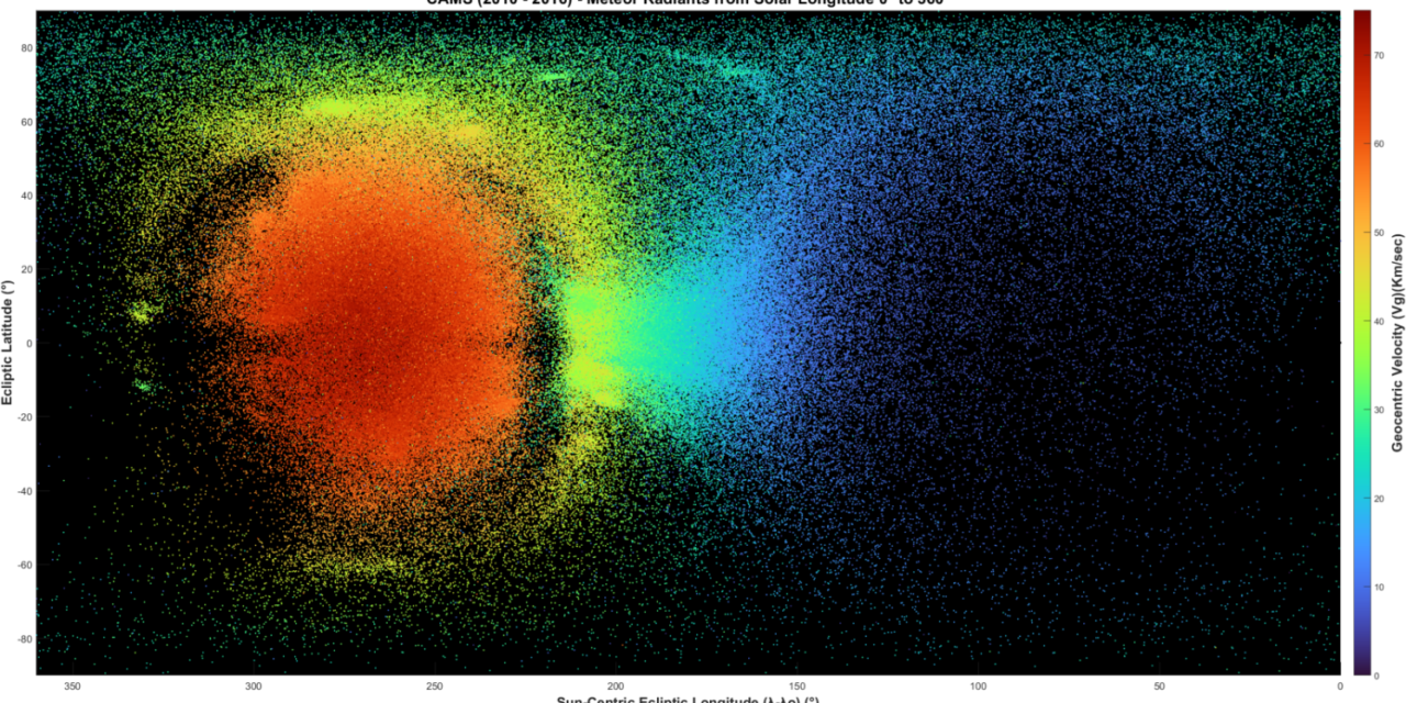
Geocentric velocity, vg:
The map of the distribution of speed (here expressed as the geocentric velocity vg) over the sky is shown as Figure 1. As one would expect, the fastest meteors are hitting the Earth head on in the direction of the Apex, while the slowest meteors are catching up on Earth in the direction of the Antapex. The velocities in between are mostly found towards the Anthelion, Toroidal ring and the poles. Because the geocentric velocity is a combination of the meteoroid velocity vector and the speed and direction of Earth, the map of Figure 1 shows that shower and sporadic meteor velocity is dependent on what part of the sky the meteor arrives from.
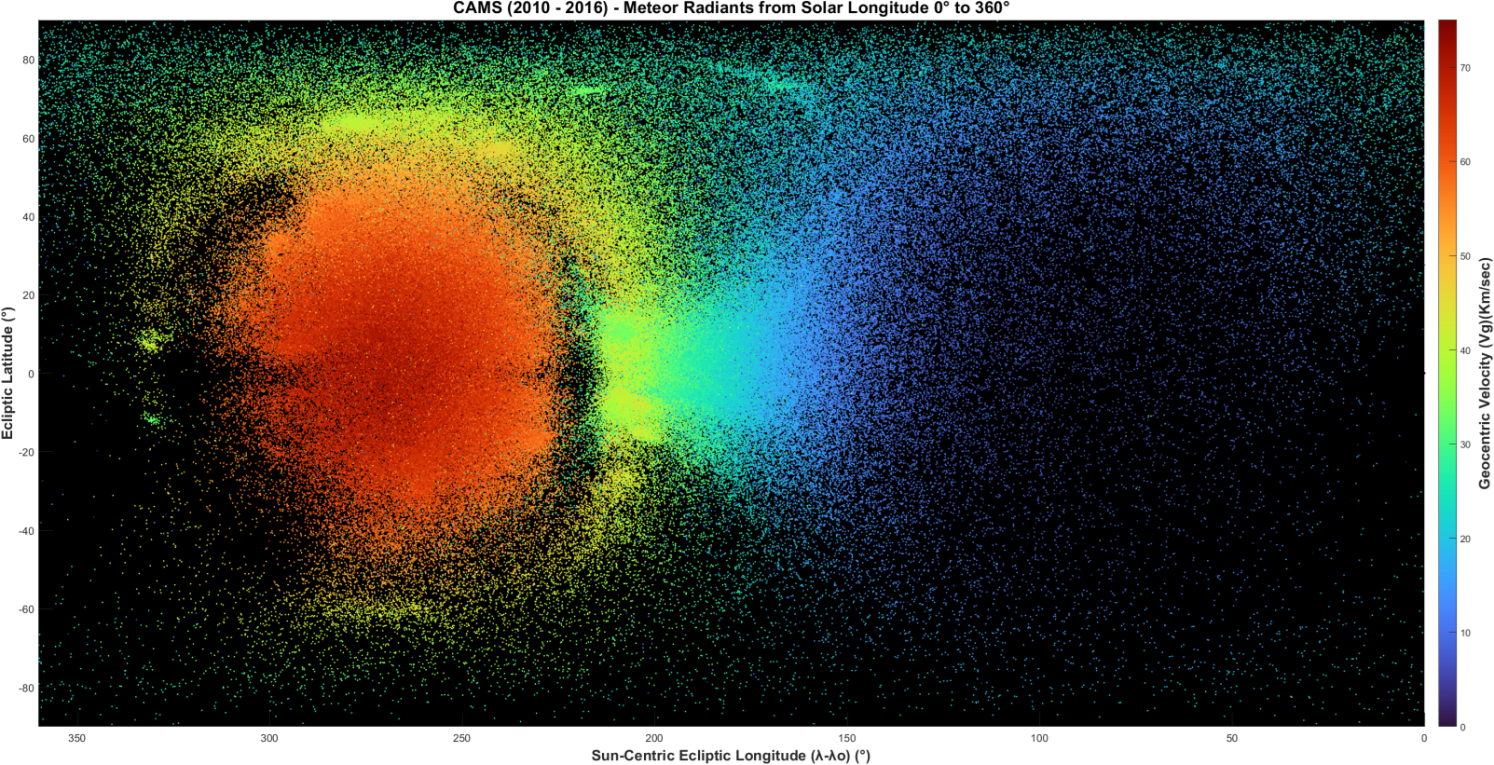
Figure 1 – Geocentric velocity vg (and Öpik vector magnitude U).
Perihelion distance, q:
This orbital element is mostly determined by the radiant direction. Figure 2 shows that the q distribution appears to emanate from the east and west transition regions, centered at 320° longitude/0° latitude and 220° longitude/0° latitude respectively. Starting from those locations with the smallest q (0 AU, red), perihelion distance increases in all directions until the largest q (1.05 AU, violet) is reached at the center of the Apex (270° longitude) and Antapex (90° longitude). The changes in q increase along relatively straight lines resulting in strong gradients and well-defined color zones. High q orbits are narrowly concentrated at the Apex and much broader at the Antapex because q increases more rapidly approaching the Apex than approaching the Antapex directions.
Notice that all shower clusters blend into the surrounding color zones, or have a similar shade within that zone. The radiants that do not blend into the background color are scattered over the Apex and extend past the northern Toroidal source, but not all the way to the pole. While less data is shown in the southern hemisphere, it is assumed to have the same distribution of these “Out of Zone Radiant(s)” (OZR) as the north. The western Anthelion and Antapex are devoid of OZR. There also appears to be a hole in the scattered OZR that coincides with the northern Toroidal source. These OZR may not be visible in the plots shown here without enlarging the view.
The interactive script revealed that these scattered OZR share high TJ parameters of ~4.3 to ~9.6 by a sample of 14 radiants from all over the Apex. All OZR appear to be in asteroid-like orbits among the otherwise dominant population of Jupiter-family comet and long-period comet orbits. However, some are in Sun-grazer comet orbits like those around the east and west transition regions.
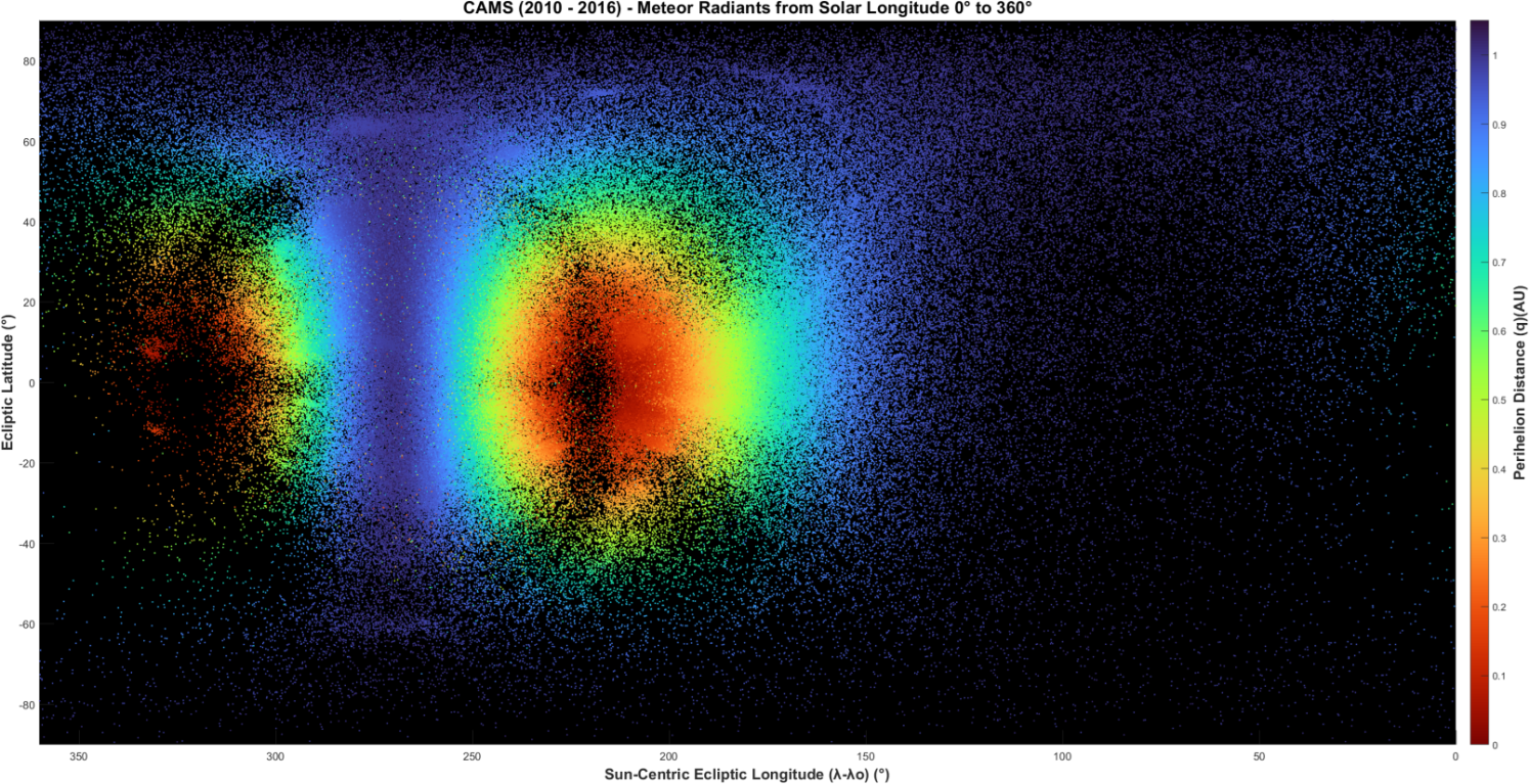
Figure 2 – Perihelion distance q.
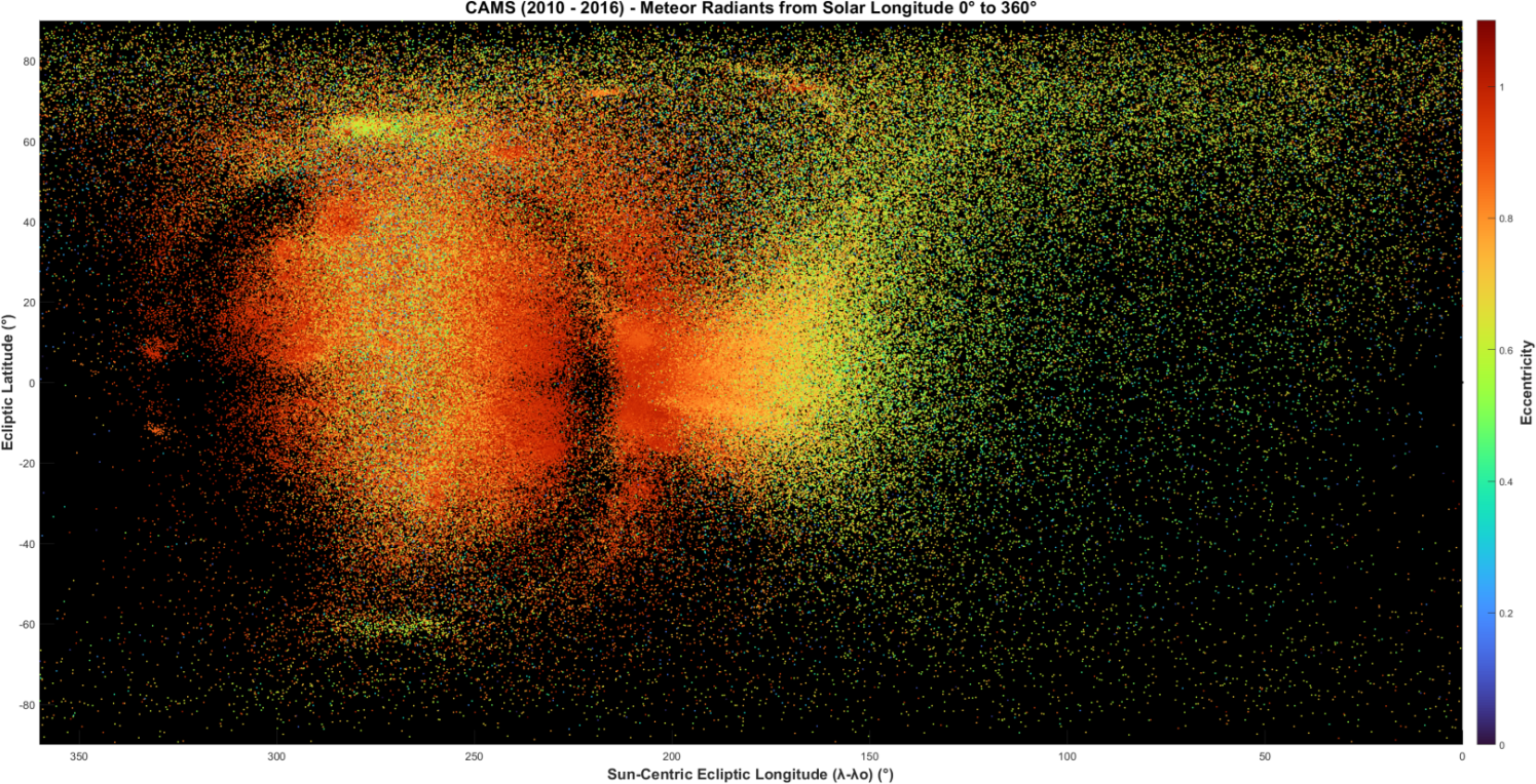
Figure 3 – Eccentricity e.
Eccentricity, e:
Figure 3 shows that the e distribution is much less organized than q and much of the distribution is mixed because this parameter strongly depends on the measured speed. The most obvious structure is the concentration of high eccentricities approaching or exceeding (due to measurement error) the value of e = 1.0 around the east and west transition regions, and up and down the Toroidal ring. The strongest gradients lead out of these regions, but break down quickly into a scattered distribution, especially approaching the Apex. The north and south Toroidal sources have distinct high e ~0.7 that stand out from the background, as does the western Anthelion source.
The Anthelion source meteoroids change eccentricity from the highest e (> 0.8) in the east to lower e (0.35 – 0.80) in the west as it becomes more diffuse in latitude approaching the Antapex. The Antapex is likewise dominated by 0.35 < e < 0.80, with few e < 0.35 and fewer e > 0.80.
A distribution of radiants resembling the Narrow Apex source in radar data (Jenniskens, 2023, p. 89) is seen when e is restricted to lower values (Figure 4) and the lower e is restricted, the narrower the Apex. Empirical measurements of the Apex width (WE) at the ecliptic were made from plots (not shown here) for e thresholds in increments of 0.10. The results suggest that from 0.0 ≤ e ≤ 0.7 the least squares fit is linear,
WE (°) = –3.07 + 64.33emax (1)
and that for 0.7 ≤ e ≤ 1.1 the least squares fit is exponential,
WE (°) = 6.24 * ln(2.69emax) (2)
where WE is the width of radiants at the ecliptic in degrees, emax is the threshold for eccentricity, and the system limiting magnitude is ~5.5. Both fit equations have high reliability R > 0.99 over their ranges.
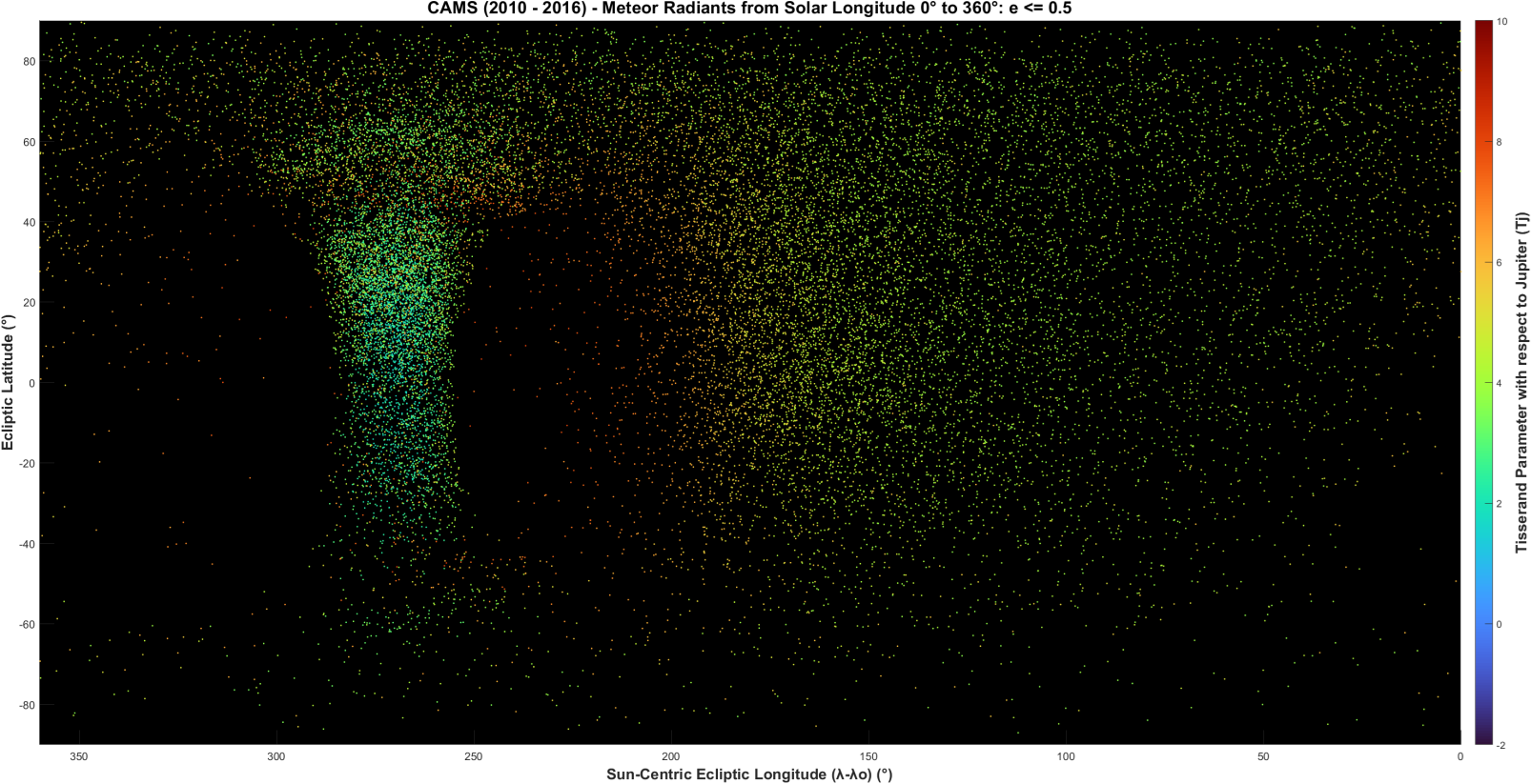
Figure 4 – Narrow Apex Source seen for e < 0.50. Colors show TJ parameters.
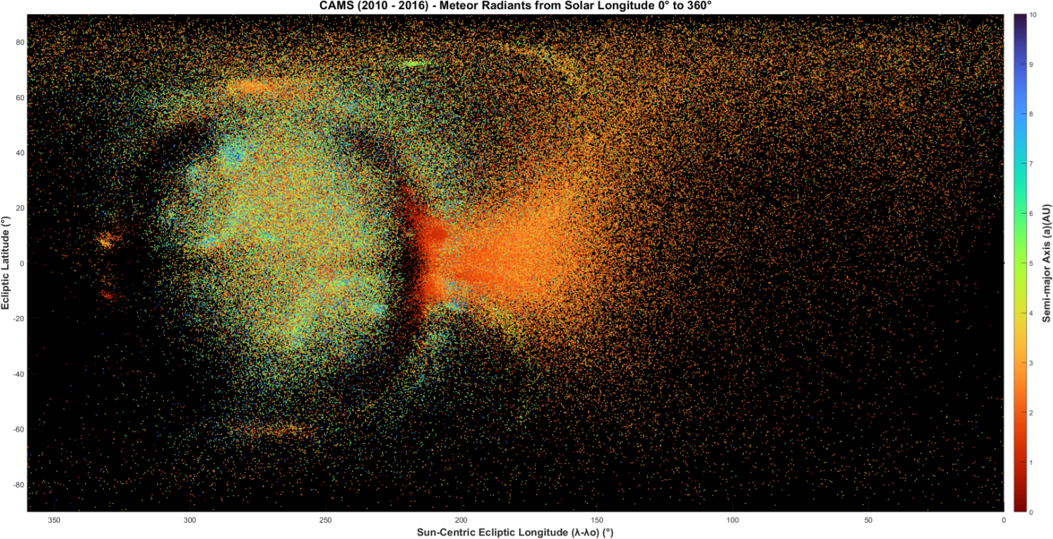
Figure 5 – Semi-major axis, a, from 0–10 AU.
Semi-major axis, a:
The semi-major axis is defined by speed also, even more so than the eccentricity. Figure 5 shows the distribution of a scaled from 0 AU to 10 AU. Like e, semi-major axis a is largely mixed, with a concentration of low-a orbits at the Anthelion side of the western transition region. The rest of the Anthelion is also composed of low a orbits, but somewhat higher than the low-a orbits at the transition region. This low-a trend continues moving west through the Antapex and Helion. The Apex and Toroidal ring are noticeably both composed of orbits with longer semi-major axes, but also contain a mix of the low-a orbits. The Toroidal sources both stand out from the Toroidal ring with low-a orbits. Some shower radiant clusters do stand out from the mixed background.
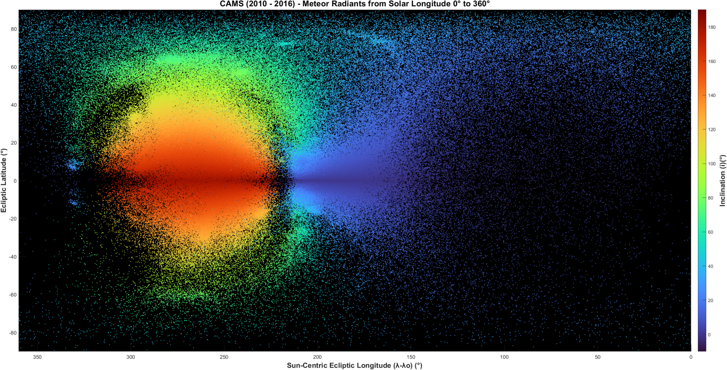
Figure 6 – Inclination i. The scale has been extended beyond 0°–180° to make the low i radiants easier to see.
Inclination, i:
Figure 6 shows that the distribution of i is quite organized like that of q, but with a different structure symmetrical about the ecliptic plane. Like q, the gradients are strong and the color zones are well defined. Shower clusters and the background both blend together in the color zones, with some small deviations like towards the Geminid radiant at around 210° longitude, +10° latitude.
High retrograde (i > 90°) orbits are centered on the Apex, and low prograde (i < 90°) orbits are centered on the Antapex source. All retrograde orbits are confined to the Apex, arriving in a cone with a base diameter of ~110°, centered at 270° longitude and 0° latitude, the Apex of the Earth’s way. This boundary is in the transition region, just inside the Toroidal ring. The rest of the sky and sources are prograde, with a thin scattering of prograde radiants among the retrograde radiants in the Apex.
Where the Anthelion meets the Toroidal ring the mean value of i increases rapidly moving up or down the ring, and levels off around i ≈ 72° at about ±40° latitude. The OZRs seen in the western transition region are all sungrazers with mixed TJ and i, and with e close to or slightly over e = 1.
Some OZR are seen in the Apex and in the western transition zone. The Apex OZR are the same as those seen in q with high TJ, but in the western transition region the TJ parameters are much lower, less than 4.0 in general, and even less than zero in some cases. Notice that, given the way the color zones are structured for i, all colors meet at the ecliptic in the eastern and western transition regions. The inclinations of radiants located there can take on a wide array of values.
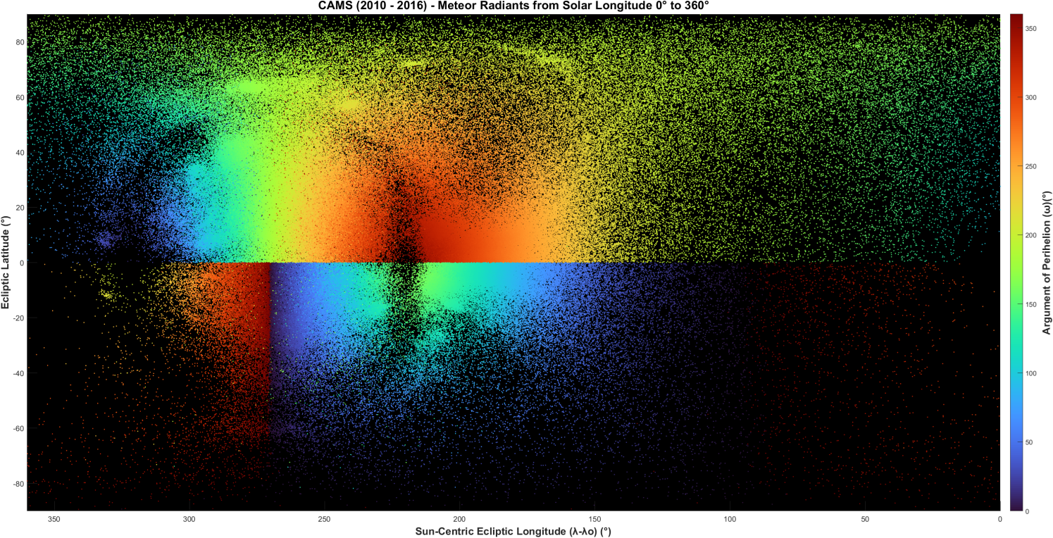
Figure 7 – Argument of perihelion ω.
Argument of perihelion, ω:
The argument of perihelion shown in Figure 7 also has a distribution that is organized although with an abrupt 180° flip at the ecliptic. The flip at the ecliptic occurs because the ascending node shifts 180° when crossing the ecliptic plane. The argument of perihelion is measured from the ascending nodal point of the nodal line, so when the ascending node shifts by 180°, so does ω. The abrupt vertical changes at 270° and 90° from red to blue and back in the southern hemisphere are actually smooth changes from 360° to 0°.
Orbits approach ω = 0°/360° in the northern transition regions, decreasing to 0° on the eastern side, and increasing to 360° on the western side. The 180° flip in the southern hemisphere means that in the southern transition regions orbits approach ω = 180° from above on the eastern side and from below on the western side. Orbits approach ω = 180° at the North Pole and ω = 0°/360° at the South Pole.
No showers stand out against these color zones, not even the Geminids. Elongated shower radiant clusters change ω according to the color zone they pass through. Only the OZRs seen against the Apex source in Figure 2 stand out against the background.
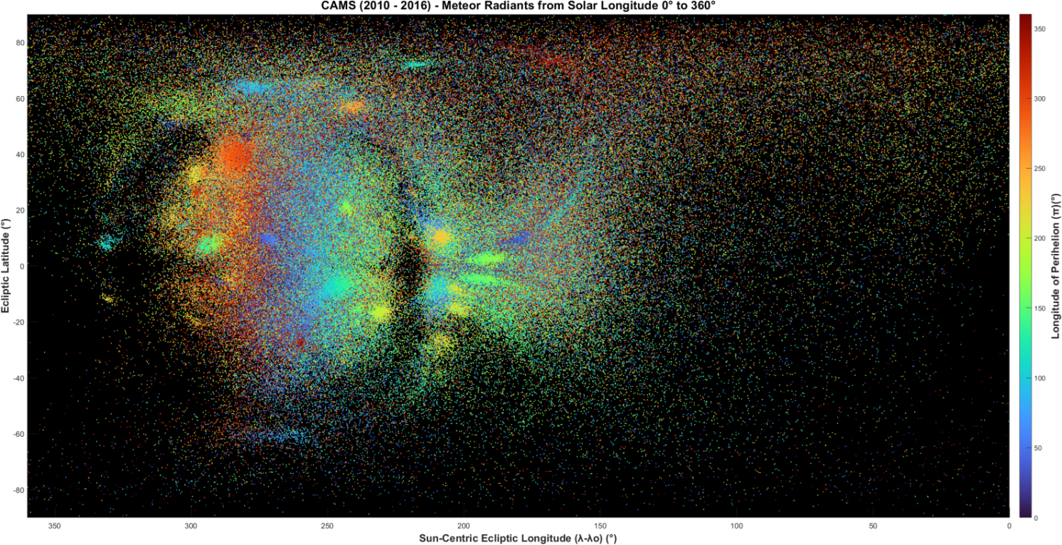
Figure 8 – Longitude of perihelion Π.
Longitude of perihelion, Π:
By itself, a plot of the ascending node Ω is not very informative, but when added to ω to make Π some things are revealed, because now showers at different times in the year are separated (Figure 8). While there are no well-defined color zones, individual shower clusters stand out in various colors against the thoroughly mixed background of the Anthelion and poles. The Antapex is also thoroughly mixed, but has no visible shower clusters.
The Apex shows a background distribution of Π that approaches 0° at the center (270° longitude), from high values on the east, and from low values on the west. Shower clusters of various colors stand out against this background variation.
The southern Toroidal source appears to contain two sets of Π values (red on the east and blue on the west). The northern Toroidal source is too obscured by the background to tell if a red component is present, but does have a blue shower cluster on the eastern side, symmetrical about the Apex of the Earth’s direction of motion (270°/0°) with the southern blue component. Both components cross over the 270° longitude line in the south, where the value of ω changes abruptly. The northern blue shower cluster is completely on the eastern side of the 270° longitude line.
4 Non-Keplerian element distributions
D criteria DN and DR are expressed in terms of the Öpik parameters U, ϕ, and cos θ (Valsecchi, et al., 1999). Here, we examine how well those parameters separate showers and their sporadic background.
Vector U:
U is the vector of the meteoroid (Öpik, 1976). The dimensionless magnitude of U is the meteoroid velocity divided by the Earth’s velocity, with a maximum ratio of 2.53. When U is scaled from 0 to 2.53 the plot is identical to the plot for vg scaled from 0 to 75 kilometers per second shown in Figure 1. The direction of U is defined by ϕ and θ, discussed below.
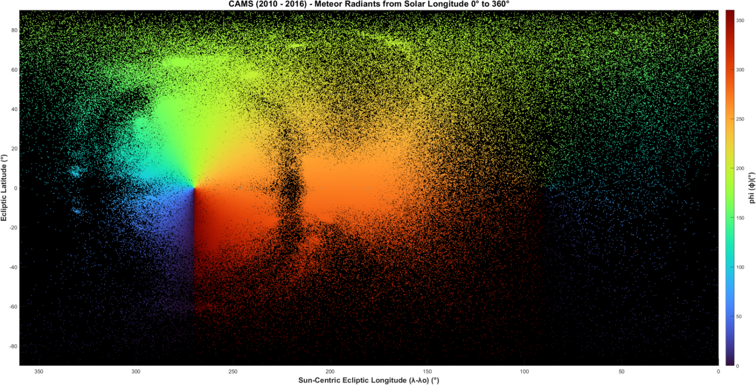
Figure 9 – Öpik variable ϕ.
Angle phi, ϕ:
Figure 9 shows phi ϕ, the angle between the plane containing the vector U and the y–z plane, where the positive y-axis is the direction of the Earth’s way, and the z-axis is normal to the ecliptic plane. The y-axis intersects the plot at the Apex (270°/0°) and the Antapex (90°/0°).
Figure 9 shows that the color zones revolve around the y-axis as the plane of vector U is rotated around the y-axis and that as an angular value ϕ changes smoothly. The difference between shower radiants and background radiants is undetectable.
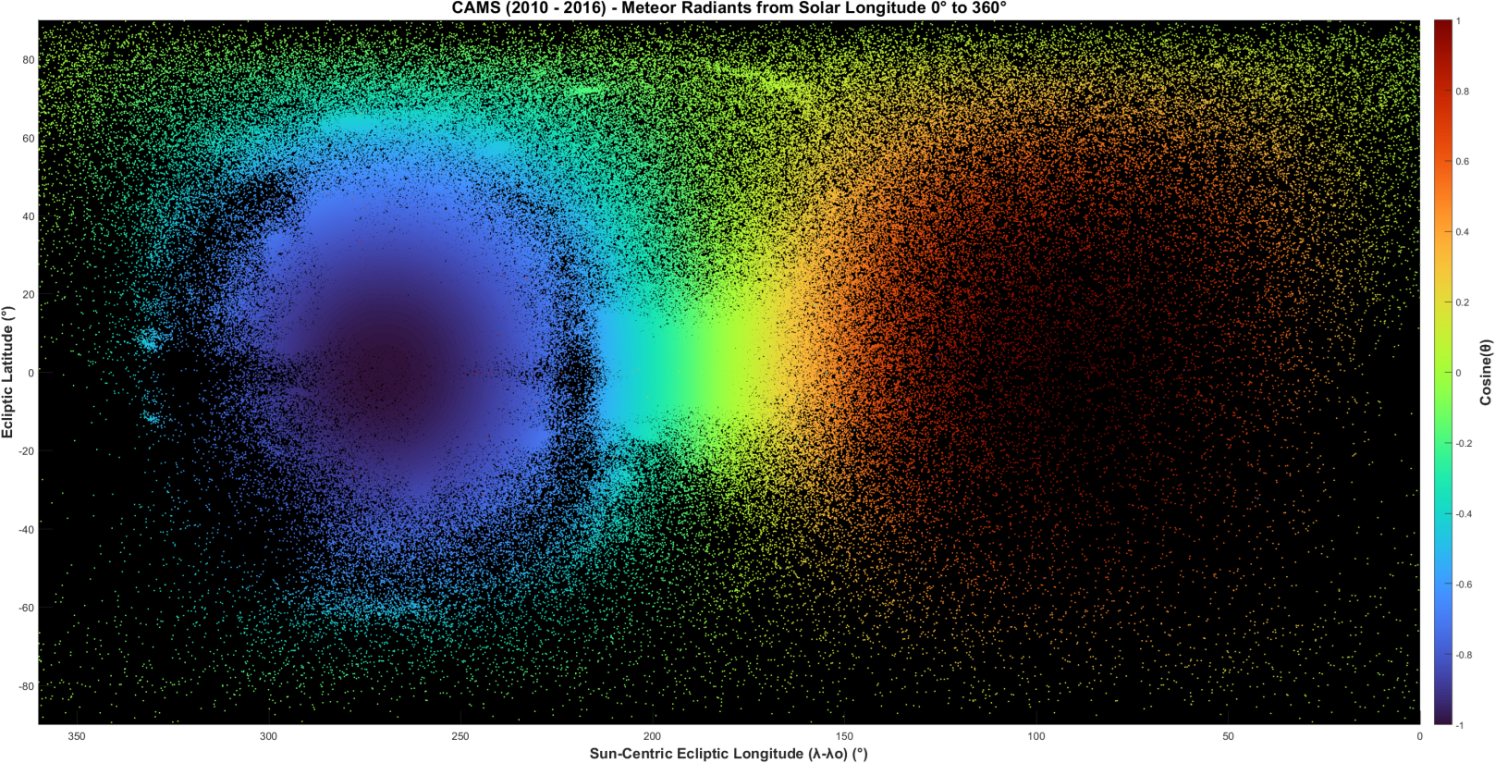
Figure 10 – Öpik variable cosine (θ).
Ratio cosine θ:
Theta θ is the angle between the vector U and the direction of the Earth’s way, the positive y-axis. In Figure 10 cosine θ is used instead of θ because cosine θ is said to be proportional to –1/a, which is the orbital energy of the meteoroid.
As an angle ratio, the color zones in the cosine θ plot are smooth, like for ϕ. Again, the difference between shower and background sporadic meteors is undetectable.
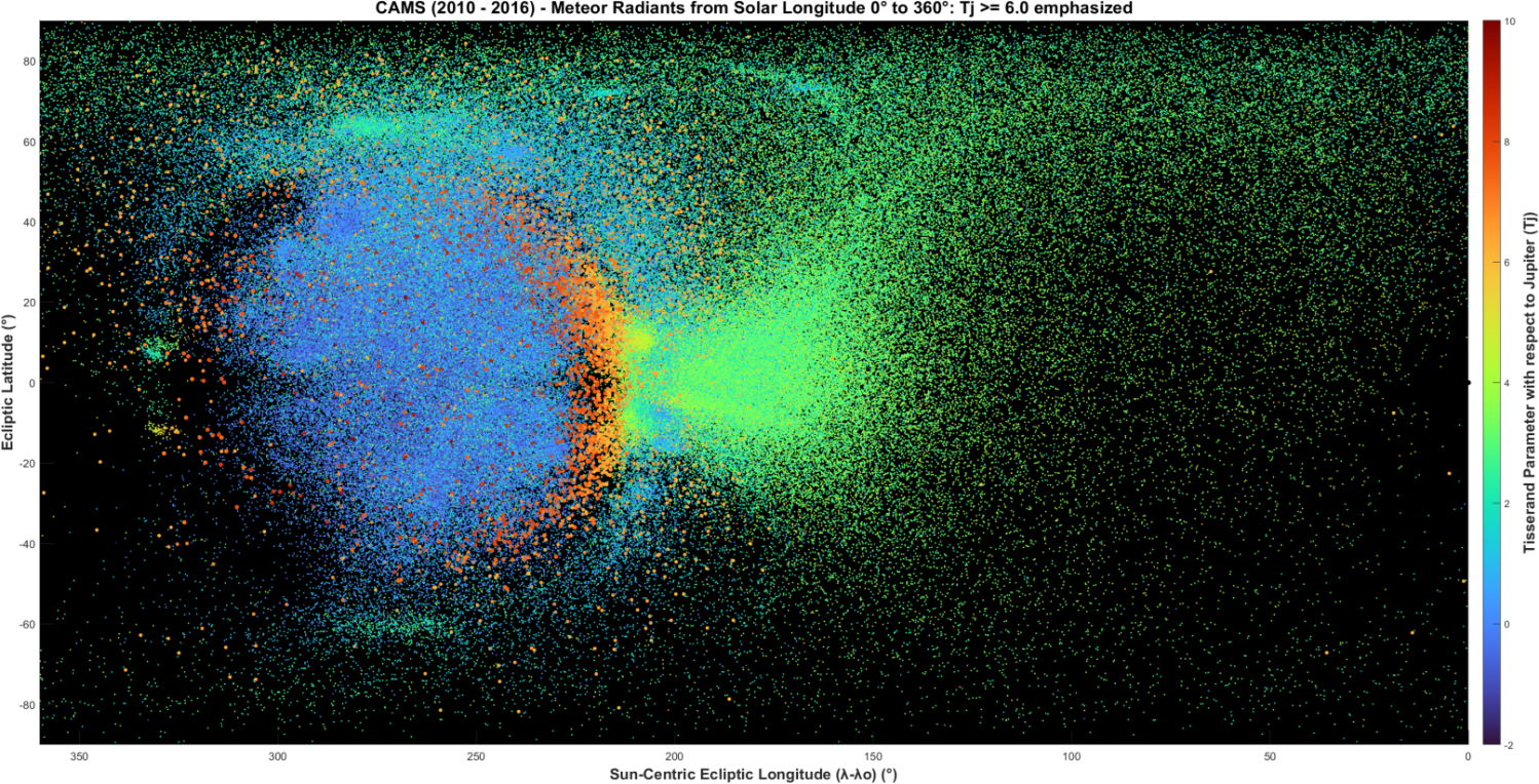
Figure 11 – Tisserand parameter with respect to Jupiter, TJ. Radiants with TJ ≥ 6.0 are plotted with larger markers. Radiants with TJ ≥ 7.0 are plotted with even larger markers.
Tisserand parameter with respect to Jupiter, TJ:
Figure 11 shows the distribution of TJ. In this plot radiants with TJ ≥ 6.0 are plotted with larger markers. Radiants with TJ ≥ 7.0 are plotted with even larger markers.
The TJ distribution is mainly divided into two regions, one of blue radiants with low TJ parameters at the Apex and Toroidal ring, and one of green radiants with middle TJ parameters at the Anthelion, Antapex, and poles. A concentration of yellow, orange, and red high TJ parameters appears in the western transition region, and presumably exist in the same way at the eastern transition region, but for lack of data due to daylight.
The Apex is dominated by low TJ parameters near zero, indicating Long Period Comet-type orbits, with occasional orbits having TJ around 1.5–2.0, in between Mellish-type and Jupiter Family Comet (JFC)-type orbits. The Toroidal ring is composed of radiants with Mellish-type orbits with TJ ~ 1.0–1.5 while the Toroidal sources have higher TJ parameters of 2.0–2.5 indicating JFC-type orbits.
It was found that radiants with TJ ≥ 7.5 are confined to the Apex, inside the transition region, but only a small fraction are in retrograde orbits. The larger the TJ threshold, the more restricted the radiants are to the center of the Apex at 270° longitude, 0° latitude. Radiants with TJ ≥ 7.0 spread wider to the just outside of the transition region. Radiants with TJ ≥ 6.0 spread even wider to the Anthelion, Helion, and the poles, but not in the Antapex.
Some of the OZR with high TJ parameters seen in Figures 2 and 11 are in the transition regions where, with low to middle eccentricities, they stand out against the red high e radiants there. They can also be seen in the voids outside the Narrow Apex Source in Figure 4.
5 Discussion
The radiant plots show that orbital elements that are mostly determined by the radiant position are distributed across the sky in organized, predictable ways that are the same for shower and sporadic meteors. The perihelion distance, inclination, argument of perihelion, and geocentric velocity are distributed in such a way that the vast majority are surrounded by similar orbital element values, and those values change in gradual and predictable ways moving across the sky.
The gradients of these orbital element values across the sky are not perfectly smooth. In the immediate neighborhood of a radiant, its adjacent neighbors can be slightly larger or smaller in any direction, but as the radiant moves further away from the original location the trends are revealed by the separate and well-defined color zones. These color zones are larger than most shower clusters. The geocentric velocity gradients are the most diverse of the above elements, but still highly constrained in a given radiant direction. It is unclear why the argument of perihelion is relatively smoothly changing towards the Anthelion source direction, compared to other sources and elements.
The distribution of eccentricity and semi-major axis are much less organized because they are mostly determined by the measured speed. The changes from one place to another are far less predictable, yet are still organized in a few ways. The highest eccentricities that approach or exceed 1.0 are concentrated around the east and west transition regions (Figure 3), similar to the lowest perihelion distances in Figure 2. In the Apex the lowest eccentricities are confined to the center, distributed in the same way as the Narrow Apex source (Figure 4), which signifies an excess of low-e orbits in radar observations.
The Öpik parameters U, ϕ, and cosine θ also exhibit a strong organization with strong gradients. U plots identical to vg and shares the same characteristics. Phi (ϕ) and cos θ vary smoothly, expressing an angle and an angle ratio, respectively. Cosine θ is thought to be a near invariant (Valsecchi, et al, 1999), but a plot of its values does not resemble that of TJ (Figure 11). The most noticeable difference is in the Antapex where cosine θ is of the highest values in Figure 10, but the highest values of TJ are located in the western transition region, and the Antapex is composed of TJ ≥ 3.0–3.5 which are still asteroid-like orbits, but not at the extremes of TJ in Figure 11.
The transition region:
The “transition region”, the void just inside the Toroidal ring, is where various transitions take place. First, it is the boundary that contains all retrograde orbits (i > 90°) within the Apex, which also contains a scattering of prograde orbits (i < 90°). Outside of this boundary all orbits are prograde. Second, the eastern and western sides at the ecliptic, where the void is at its widest, contain the Sun-grazer orbits, with the exception of the scattered radiants in the Apex that are in asteroid-type orbits with high TJ and small q. The closer a radiant is to the center of this void (~220° longitude, 0° latitude, for the western side) the closer the meteoroid orbits to the Sun. One can think of the Sun as being gravitationally located at these points as q approaches zero. At these same locations, inclinations become chaotic and take on a wide range of values.
These two parts of the transition region are also the epicenters of the highest eccentricities, approaching and exceeding 1.0. Outside of these regions eccentricity is largely mixed, with the lowest eccentricities in the Apex concentrating toward the center (270° longitude).
There are concentrations of high TJ parameters (TJ > 6.0) around these regions that tend toward the inside (Apex side) of the transition regions. TJ parameters ≥ 7.5 are completely confined to the Apex inside the transition region boundary.
The argument of perihelion ω approaches 0°/360° in the northern hemisphere, and 180° in the southern hemisphere at these regions. These regions are where perihelion occurs at or near Earth, and is ascending there, or where perihelion occurs on the far side of Earth’s orbit and is descending there. In this latter case the semi-major axis must be ≤ 1 AU for the meteoroid orbit to intersect the Earth’s orbit but have q on the other side of the nodal line. These radiant orbits are gathered at the Anthelion (and presumably Helion as well) side of the transition region (Figure 11).
The Out of Zone Radiants (OZR) seen in the perihelion distance plot, Figure 2, are also seen in the argument of perihelion plot. The same OZR can be seen in the eastern and western transition regions of the eccentricity plot, the only areas that are not mixed, and less so in the vg and TJ plots. These OZR are scattered over the Apex, eastern Anthelion, and western Helion sources while the Antapex lacks them completely. All have high TJ parameters putting them in asteroid-like orbits. The higher the TJ parameter is, the more confined to the Apex of the Earth’s way do the radiants occur and that for TJ ≥ 7.5 the radiants are confined to the Apex source. The OZRs do not show up in the Opik parameter plots, or in the mixed plots like a, or the Apex distribution of e.
Implications for the use of D criteria:
D criteria are mathematical formulae that describe the similarity between two orbits and are intended to separate shower meteoroids from the sporadic meteoroid background. Most are based on orbital elements q, e, i, ω, and Ω.
It can be seen from the plots that q, i, and ω have distributions that change gradually and more or less smoothly over large areas, forming color zones that are larger than the typical shower radiant cluster, and that shower radiant clusters do not differentiate from these color zones. However, separated over a narrow time span typical of shower durations (a few degrees up to tens of degrees) shows that these elements do stand out from the sporadic background, especially Π = ω + Ω, because it doesn’t have the 180º flip of ω and Ω separately when crossing from northern to southern hemisphere.
The plots of a and e (Figure 5 and 3) shows a mix of values over most of the sky, but a concentration approaching (and exceeding due to measurement error) e = 1.0 is seen at the eastern and western transition regions.
The similarity of orbital elements in different directions at the sky on a given date demonstrates that using sufficiently small thresholds is essential for orbit shape D criteria to be able to differentiate shower radiants from background radiants. Even then, the likelihood of some sporadic pollution is relatively high. The same is true for D criteria that use the near-invariant Öpik parameters, namely DN and DR (Valsecchi, et al, 1999). The velocity parameter U is identical in distribution to vg, and the changes in plots for ϕ and cosine θ being angular and angular ratios, respectively, are smoother than the changes in q, i, and ω, with absolutely no differentiation between shower and background.
6 Conclusion
Meteor orbital elements (q, i, ω) that are mostly determined by the radiant direction are distributed in Sun-centered ecliptic coordinates in a manner that is independent of the time of year. Orbital elements determined by the entry speed (a, e) show a less organized pattern across the sky. Time (solar longitude) correlates strongly with the node Ω.
Several orbital elements and non-Keplerian parameters have all-sky distributions that do not differentiate between shower radiants and background sporadic radiants. Small thresholds are needed for D criteria to identify orbits that are similar.
When viewed over the whole year, meteor showers stand out best in maps of Π = ω + Ω, because adding the element of time to the argument of perihelion parameter separates showers that occur at different times in the year.
References
Jenniskens P., Baggaley J., Crumpton I., Aldous P., Pokorny P., Janches D., Gural P. S., Samuels D., Albers J., Howell A., Johannink C., Breukers M., Odeh M., Moskovitz N., Collison J. and Ganju S. (2018). “A survey of southern hemisphere meteor showers”. Planetary Space Science, 154, 21–29.
Jenniskens P. (2023). Atlas of Earth’s Meteor Showers. Elsevier, Amsterdam, p. 130.
Koukal J. (2016). “Results of the EDMOND and SonotaCo united databases”. eMetN, 1, 20–23.
Koukal J., Srba J., and Lenža L. (2024). “EDMOND v5.05”. eMetN, 9, 15–23.
Molau S., Rendtel J., (2009). “A Comprehensive List of Meteor Showers Obtained from 10 Years of Observations with the IMO Video Meteor Network”. WGN, the Journal of the IMO, 37, 98–121 and back cover of WGN 37:5.
Opik E. J. (1976). Interplanetary Encounters. Elsevier, Amsterdam.
SonotaCo (2009). “A meteor shower catalog based on video observations in 2007-2008”. WGN, the Journal of the IMO, 37, 55–62.
Valsecchi G. B., Jopek T. J., and Froeschle C. (1999). “Meteoroid stream identification: a new approach- I. Theory”. Monthly Notices of the Royal Astronomical Society, 304, 743–750.

