Abstract: The Global Meteor Network completely covered the outburst of the meteor shower related to 73P/Schwassmann-Wachmann 3. The peak activity was recorded by camera operators in Western America when the radiant was at its culmination. The analysis of the observations shows a very important fact; the meteoroids are very porous. We can confirm the meteoroids are spread centered at the perihelion of the comet and along with the orbital plane of the comet.
The faint meteor shower observed in 1930 moved southward but we confirmed the radiant of this event moved northward. TAH (#0061) in the meteor shower database (SD) of the IAU meteor data center is very dispersed and these meteoroids are thought to be rather solid ones. It seems appropriate to give a new name to this meteor shower.
1 Introduction
73P/Schwassmann-Wachmann3 broke into pieces in 1995 and many investigators predicted the released dust would encounter the Earth in 2022. The Global Meteor Network covered this opportunity very successfully and we have valuable data on the outburst. Details about the methodology used by GMN have been published before (Vida et al., 2019; 2020; 2021). This is the first-time detailed observations of the debris from 73P/Schwassmann-Wachmann3 have been obtained because we have poor information on meteors produced by dust from this comet.
2 History
2.1 Japanese observation in 1930
The first and only witness is Nakamura’s faint meteor shower in 1930 (Nakamura, 1930). Japanese researchers scheduled the observational program for observations immediately after the discovery of 73P/Schwassmann-Wachmann3. Nakamura started observations from May 24 before the expected maximum and witnessed many very faint meteors during the program till June 19. He wrote, “When a specially limited area of the heavens (some five degrees square) is watched with the utmost caution, considerable numbers of faint meteors would be suspected” and “The observation of faint meteors usually causes considerable fatigue of the eyes; the author, therefore, works, mostly for 30 minutes, or at most, 60 minutes”. He noticed the radiant southward drift though there were discussions then whether a meteor shower radiant drifted or not. Many others were not able to detect such faint meteors except one amateur.
Komaki could not detect any meteors from 73P/Schwassmann-Wachmann3 in 1935 (Komaki, 1935) and we have no certain witness about any activity till photographic research became available.
2.2 Photographic tau-Herculids
The name of tau-Herculids given in the IAU Meteor Data Center Shower Database (SD) seems curious because the listed radiant point locates in Boötes according to the reference (Lindblad, 1971). Southworth and Hawkins named an activity detected by their statistical methods as τ-Herculids (Southworth and Hawkins, 1963), and Lindblad thought his No.168 stream can be identified with their τ-Herculids. Two types of research were based on different meteor databases; Southworth and Hawkins use the ‘short trail method’ and Lindblad uses the ‘graphical reduction’. Koseki confirmed that both kinds of research are identical; the underlined numbers or marked in italics in Table 1 to 3 are common meteors. He analyzed all types of photographic databases including former Soviet data and found a cluster MK-49 (Koseki, 1982). τ-Herculids have only two meteors in the first report but 18 meteors in the third are sufficient in number to confirm there is some meteor shower activity.
A meteor shower search using the D-criterion (DSH; Southworth and Hawkins, 1963) finds sometimes a ‘shower’ beyond our common sense. In Figure 1 crosses are video meteor radiants, circles are photographic radiants, circles filled with red are members of MK-49, and red squares are June Bootids (JBO, #0161). Although MK-49 is limited by DSH < 0.15, member radiants are spread all over the chart. Interestingly, several candidates of JBO #0161 are shown in this plot as a compact group.
Table 1 – First report of τ-Herculids by Southworth and Hawkins (1963).
| Time | a (AU) |
e | i (°) |
Ω (°) |
π (°) |
α (°) |
δ (°) |
v∞ (km/s) |
|
| 53 June 20.35000 | 2.07 | 0.521 | 28.9 | 88.7 | 291 | 258.6 | +50.4 | 21.2 | H2-7920 |
| 54 June 25.24461 | 2.81 | 0.642 | 21.3 | 93.1 | 286.2 | 237.8 | +46.4 | 18.8 | H2-12711 |
| Mean values | 2.44 | 0.582 | 25.1 | 90.9 | 288.6 | 248.2 | +48.4 | 20 |
Table 2 – Second report of τ-Herculids by Lindblad (1971). Identification: Southworth-Hawkins, Comet 1930VI.
| Duration | αR (°) |
δR (°) |
vg (km/s) |
q (AU) |
a (AU) |
e | i (°) |
ω (°) |
Ω (°) |
π (°) |
| May19 – June14 | 228 | +40 | 18 | 0.97 | 2.695 | 0.633 | 18.6 | 204.2 | 71.9 | 276.1 |
Harvard serial no.: 3335, 4103, 4106, 4108, 4112, 7692, 7820, 12142, 12161, 12355, 12378, 12398, 12470, 12513.
Table 3 – Third report of τ-Herculids by Koseki (1982).
| No. | αR (°) |
δR (°) |
λ–λʘ (°) |
β (°) |
vg (km/s) |
q
(AU) |
e | i (°) |
ω (°) |
Ω (°) |
N |
| MK-49 | 228.7 | +40.7 | 130.4 | +55.2 | 14.8 | 0.979 | 0.625 | 19 | 201.3 | 75.9 | 18 |
Members: H1-7692, H1-3335, H1-12142, H1-12161, H1-12355, H1-12378, H1-12398, H1-12513, H1-4106, H1-4108, H1-4112, H2-12711, H3-4103, H3-12399, H3-7820, H6-40379A, D2-570212, K1-39.
Table 4 – Radiant density along with the distance from the converged center.
| r (°) | 1 | 2 | 3 | 4 | 5 | 6 | 7 | 8 | 9 | 10 |
| N | 583 | 487 | 208 | 95 | 29 | 24 | 7 | 18 | 10 | 13 |
| Density | 185.6 | 51.7 | 13.2 | 4.3 | 1 | 0.7 | 0.2 | 0.4 | 0.2 | 0.2 |
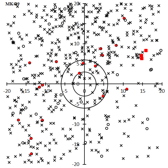
Figure 1 – The radiant distribution around TAH; red circles are members of MK-49 (compatible with TAH in the SD), black circles are photographic radiants not member of MK-49, crosses are video radiants (SonotaCo net 2007–2021) , red squares correspond to JBO (#0161) of the SD.
3 GMN observations in 2022
3.1 Data selection method
As we discussed in the former section, meteoroids of this meteor shower are spread widely, but the tau Herculids we investigate here is a young and very compact component. It seems not appropriate to adopt DSH < 0.15 to select TAH members in the GMN database or even worse to identify using the radiant distribution for instance with a distance from the center less than 20 degrees.
There are two ways to select members of a meteoroid stream. One is the radiant-based method, and another is the orbit-based method. We get meteor data in a 4th-dimensional space: radiant point (α, δ), time of observation (λʘ), and geocentric velocity (vg). We can use these data and convert them to orbital elements: eccentricity (e), distance of perihelion (q), inclination (i), argument of perihelion (ω), and node (Ω). These two sets of data are convertible to each other, and we can select any set to analyse τ-Herculids. The author chooses the radiant-based method because the orbit-based method seems superior in the case of asteroid and comet positions which are determined precisely with errors less than a few arc seconds.
We start with the initial data set: 63° < λʘ < 73°, (λ–λʘ, β) = (125°, +32°). Figure 2 (left) gives the initial radiant distribution. A tailpole-like figure is made by the radiant drift and we estimate it using the regression analysis. We plot the data in (λʘ, x), (λʘ, y), and (λʘ, vg) and analyze them by linear regression. We select meteors within 10 degrees distance from the center estimated by intermediate results and repeat this process until it converges. An example of the final converged results of (λʘ, y) is shown in Figure 3. The radiant distribution of TAH resulted in Figure 2B and we realize that the tau Herculid radiant is compact (see Table 4). Five observations of 2021 are included in this table. We select 1278 radiants within 3 degrees from the center as τ-Herculids members and use them in the following analyses.
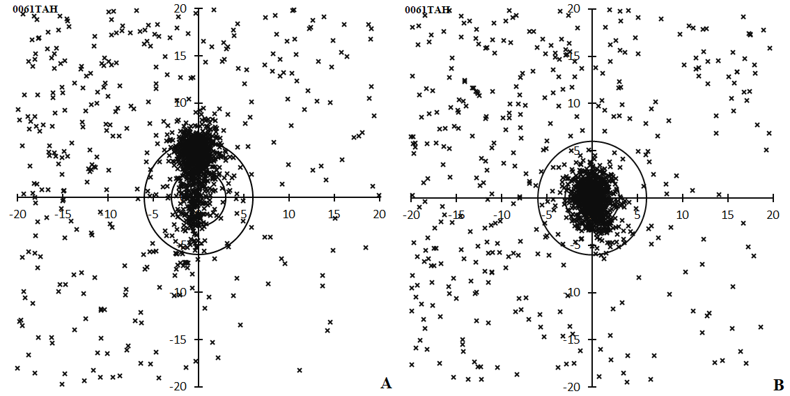
Figure 2 – Radiant distribution of video meteors (GMN) centered at (λ–λʘ, β) = (125°, +32°) between 63° < λʘ < 73°. (A, left); initial distribution, (B, right); the result after that the iterative process converged.
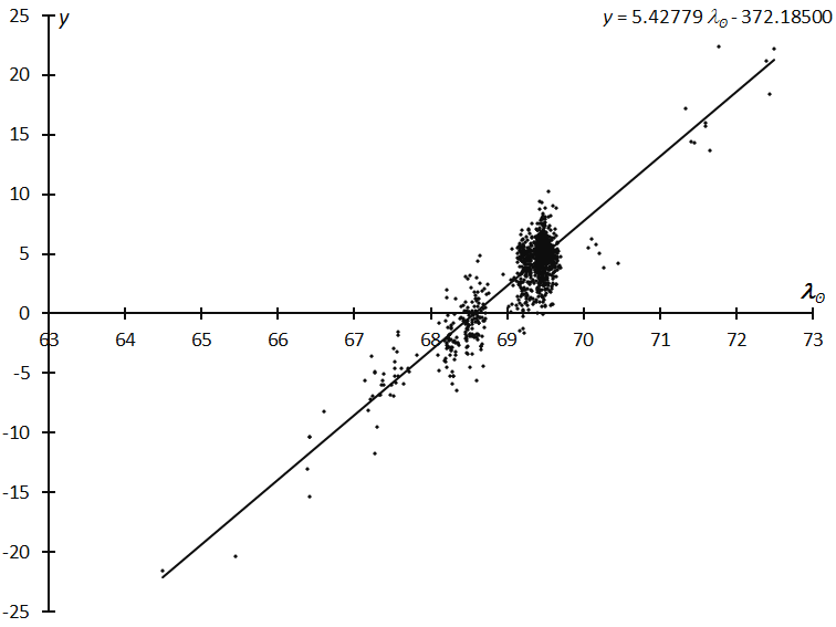
Figure 3 – Example of the linear regression analysis. The final converged results of (λʘ, y) after 9 steps of the iteration. The largest group of the data indicates the maximum and the preceding groups suggest the shower activity starts 2 days before the maximum, May 29, at the latest.
3.2 Radiant distribution
We note the final radiant distribution (Figure 2B, right) shows the elongated shape yet although the iteration converged. It is necessary to check whether the regression analysis is insufficient, or if the elongated shape is real. Figure 4 compares the radiant distributions for three periods: 63.0° < λʘ < 69.0° (left), 69.0° < λʘ < 69.5° (middle) and 69.5° < λʘ < 73.0° (right). The radiant distribution around the maximum (Figure 4B, middle) proves the elongated distribution is real because the period of this figure is short enough to avoid the radiant drift; the regression analysis is properly done. The elongated distribution is peculiar for this meteor shower (see section 3.6 Extent of meteoroid stream).
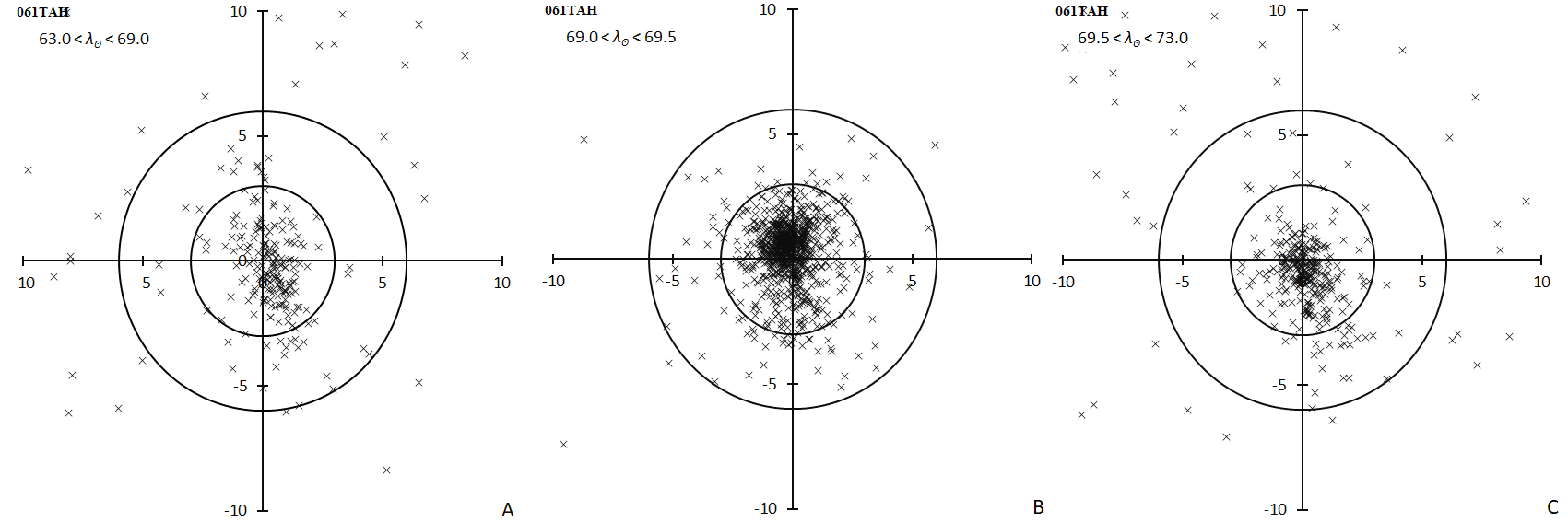
Figure 4 – Radiant distribution of video meteors (GMN) centered at (λ–λʘ, β) = (125°, +32°). (A); 63.0° < λʘ < 69.0°, (B); 69.0° < λʘ < 69.5°, (C); 69.5° < λʘ < 73.0°.
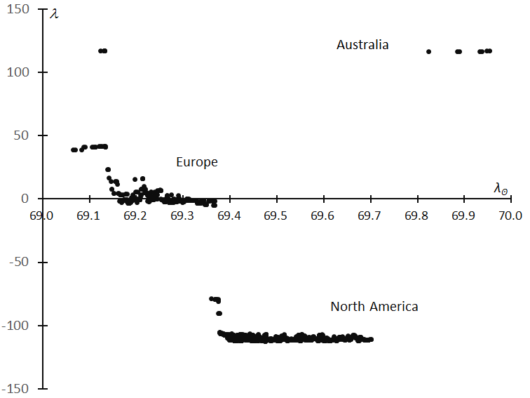
Figure 5 – Moving median of the geographic longitude λ of the begin point of the meteor paths in bins by 10 in function of time (λʘ). Observations around the maximum are linked from Europe to Canada and America.
3.3 Activity profile
The distribution of the observations in Figure 3 is intermittent and indicates GMN could not catch the activity profile of τ-Herculids continuously, but Figure 5 shows GMN members in Europe and North America covered the activity around the maximum successfully. Figure 6 gives the detail of the activity profile of the tau Herculid maximum; we estimate the number of meteors per time bin of one solar longitude using the period of 30 meteors, smoothed by the sliding average. The τ-Herculids reached their maximum at λʘ = 69.417° (May 31, 04h14m UTC) with 13580 meteors per solar longitude: HR = 565 or about 10 τ-Herculid meteors per minute. The maximum is very short, and the HR decreased to 200 after 2 hours.
The depression around λʘ = 69.3°~69.4° seems to be caused by the scarce number of observations between Europe and Western America. The ephemeris for the τ-Herculid outburst was confirmed by observers in Western America as expected.
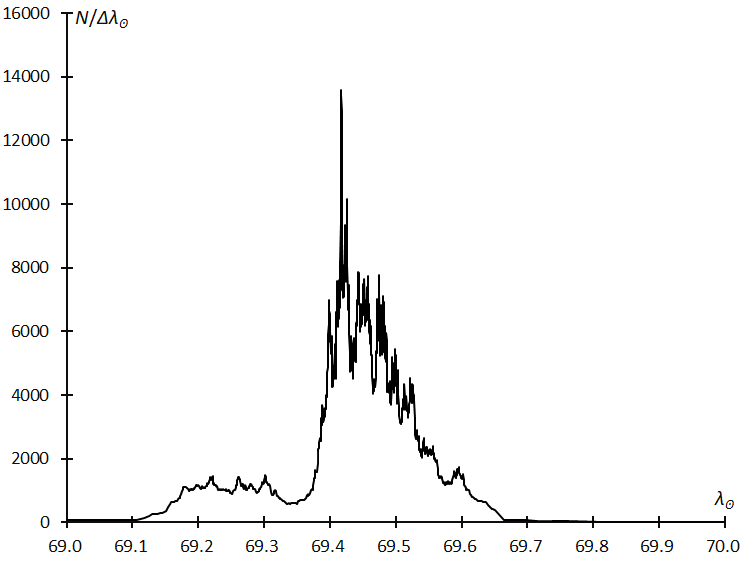
Figure 6 – Profile of the outburst obtained by the GMN. The ordinate is the estimated number of meteors per one solar longitude from the time span of 30 video meteors.
3.4 Observational restriction
3.4.1 Observational location and elevation angle
GMN camera operators pursued the tau Herculid activity but the elevation angle altered as Figure 7 shows; we perceive several peaks, indicating that several observational groups exist. The radiant of the τ-Herculids was descending under 30 degrees and the morning dawn hindered European observers before the maximum (λʘ = 69.417°). Such conditions cause an apparent decrease in τ-Herculid rates.
On the other hand, evening twilight ends, and the radiant of the τ-Herculids rises to its culmination for observers in North America. But, after λʘ = 69.7°, the radiant goes down, and the morning dawn hindered observations from Europe. The activity profile of the τ-Herculids after λʘ = 69.7° is lower than the reality.
It is worthwhile to note that the zenith attraction for the τ-Herculids is larger than for the usual meteor showers we observe. Figure 8 shows the difference between the apparent radiant and the geocentric radiant during λʘ = 69.4°~69.7°, which is for observations from North America. The difference is minimum at the radiant culmination and it becomes larger as the radiant goes down. The difference widens more than 10 degrees when the elevation of the radiant becomes lower than 40 degrees; visual observers encounter difficulties in such cases, to classify a meteor whether sporadic or not without careful observations.
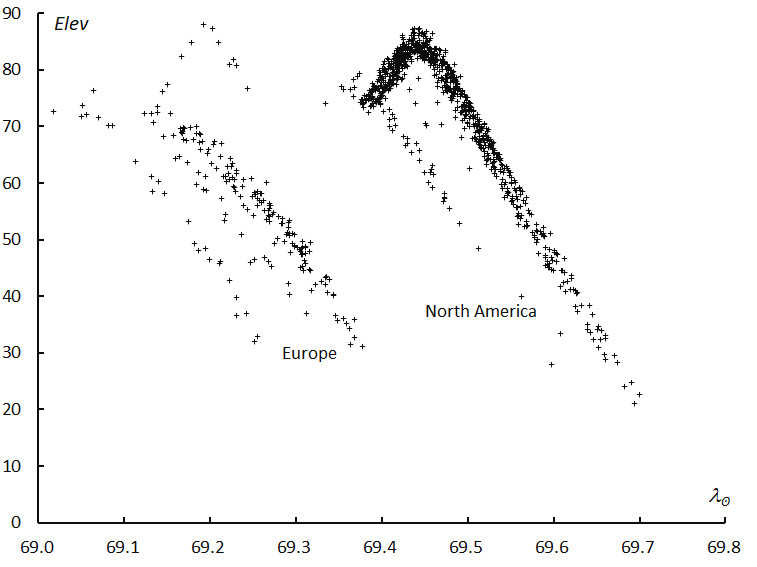
Figure 7 – Elevation angle of meteors of the outburst. Observations continued from Europe to Canada, Midwestern of USA, and Western USA.
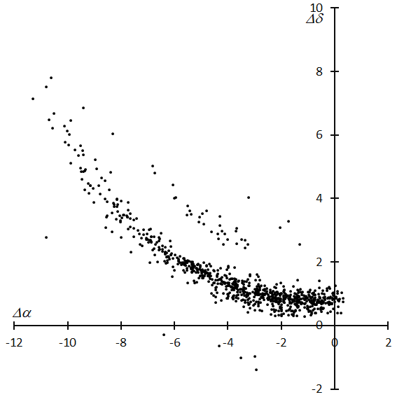
Figure 8 – Difference between the apparent radiant and the geocentric radiant. Left is east and top is north. When the geocentric radiant goes down, the apparent radiant seems to remain.
Table 5a – The positional error distributions of the classified τ-Herculids.
| α ± | 0 | 0.1 | 0.2 | 0.3 | 0.4 | 0.5 | 0.6 | 0.7 | 0.8 | 0.9 | 1 | 1.1 | 1.2 | 1.3 | 1.4 | 1.5 | 1.5< |
| N | 0 | 39 | 140 | 166 | 175 | 134 | 111 | 101 | 77 | 57 | 52 | 55 | 35 | 31 | 33 | 15 | 57 |
| δ ± | 0 | 0.1 | 0.2 | 0.3 | 0.4 | 0.5 | 0.6 | 0.7 | 0.8 | 0.9 | 1 | 1.1 | 1.2 | 1.3 | 1.4 | 1.5 | 1.5< |
| N | 0 | 42 | 150 | 169 | 179 | 142 | 107 | 96 | 71 | 66 | 61 | 42 | 27 | 31 | 29 | 16 | 50 |
Table 5b – The velocity error distributions of the classified τ-Herculids.
| vg ± | 0 | 0.1 | 0.2 | 0.3 | 0.4 | 0.5 | 0.6 | 0.7 | 0.8 | 0.9 | 1 | 1.1 | 1.2 | 1.3 | 1.4 | 1.5 |
| N | 6 | 313 | 364 | 225 | 131 | 87 | 62 | 23 | 21 | 24 | 13 | 5 | 3 | 1 | 0 | 0 |
3.4.2 Observational errors and the spread of meteoroids
We get the corrected radiant distribution for the tau Herculids from the regression analysis (see Figure 2B), Table 4 gives the radiant density per square degree. It is clear that the radiant distribution from about 6 degrees away from the center becomes diffuse enough to merge with the sporadic background. It is necessary to confirm whether this distribution exhibit the real spread of meteoroids or is mainly influenced by observational errors.
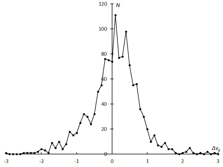
Figure 9 – Residual distribution of geocentric velocity after the regression analysis.
Table 5a shows the errors for α and δ given in the GMN database. Observational errors are estimated to be less than 1 degree in both α and δ. The radiant distribution in Table 4 is much larger than in Table 5a. It could be suggested that Table 4 represents the spread of the meteoroids themselves and not observational errors. It could be partially the case (see section 3.6 Extent of meteoroid stream). The activity profile (Figure 6) is so sharp that meteoroids are distributed tightly because they are very young. It is suggested that the radiant distribution (Figure 5A) is caused mainly by errors, what means that the error estimation of the GMN might be too small.
For the velocity determination, we can suggest a similar conjecture that the error estimates on the geocentric velocity might be too small. Figure 9 displays the residual distribution of the geocentric velocity after the regression analysis and suggests a wider spread than the error estimations given by GMN (Table 5b).
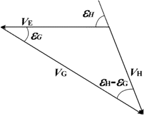
Figure 10 – Scheme of the meteoroid motion (vh), Earth’s motion (ve), and the motion of the meteor viewed from Earth (vg).
But the tau Herculids are very special as we see in Figure 8. The tau Herculid meteor shower is very slow because its meteoroids collide with Earth from behind. Figure 10 displays the ordinary relation of the meteoroid motion (vh), Earth’s motion (ve), and the motion of the meteor viewed from Earth (vg). Their relations can be expressed in the following formula:
This formula indicates that when vh changed linearly, vg would not change linearly. We can estimate the apparent radiant spread of the tau Herculids as about 2.5 times larger than the apex source meteor showers by this formula. If we considered this influence, the error estimates of GMN would be exact.
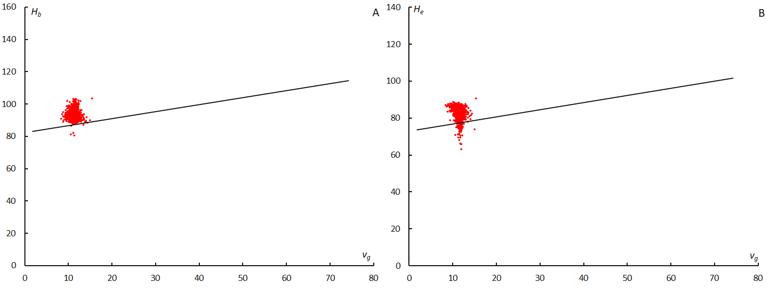
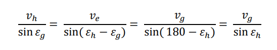
Figure 11 – Beginning height Hb of the tau Herculids (graph A, left) and end height He (graph B, right). Black lines are the approximate velocity of other meteors that appeared during the survey (63° < λʘ < 73°).
Figure 12 – Relation of beginning height to velocity outside the atmosphere (Ceplecha, 1968). TAH in red indicates the results of this research.
3.5 Distinctive nature of tau Herculids meteoroids
3.5.1. Beginning height and velocity
τ-Herculid meteoroids start to radiate and fade away at higher elevations than other meteoroids (Figure 11A and 11B). We know that slower meteors ablate lower, but τ-Herculid meteors ablate higher than others with the same velocity. Ceplecha (1968) investigated the relation of beginning height to velocity outside the atmosphere and found three ridges of maximum density of points (Figure 12). Cook considered τ-Herculids in Ceplecha’s class as ‘A or lower’; it is necessary to note the ordinate of Ceplecha’s figure (Figure 12) is inverse, and the lower height is displayed at the top in the figure. The beginning height of τ-Herculids expressed in Figure 11A is indicated as ‘TAH’ in red in Figure 12. It could be described as ‘above C’ according to the style of Cook. Other showers which Cook classified as ‘above C’ are the October Draconids, Leonids and Monocerotids. Cook (1973) wrote: “association of Ceplecha’s Class C with the residue of the ice-impregnated surface of a cometary nucleus after sublimation of the ices, and of Ceplecha’s Class A with the core of a cometary nucleus’. Omission. ‘Furthermore, the density of Class A meteoroids (1.2 g cm^–3) is so close to that of Type I carbonaceous chondrites (2 g cm^–3).’ Omission. ‘The recovery of Comet 1930 VI, Schwassmann-Wachmann 3, at its return in 1979 is urged since it is the only available comet producing a shower (τ Herculids) of Class A”. It is clear that the 2022 outburst of the τ Herculids is formed from new cometary particles but the photographic, formerly recorded τ Herculids could be from another asteroidal body or ancient cometary nuclei. We find a new question on the origin of the former τ Herculids (fTAH).
Cook classified Geminids as class B. We will compare the new τ Herculids (nTAH) with the Geminids in the following sections.
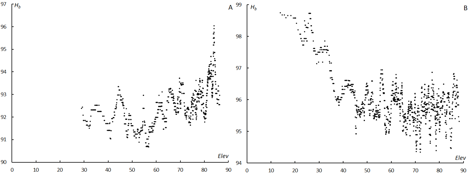
Figure 13 – Beginning height and elevation angle. (A); τ Herculids, (B); Geminids.
3.5.2. Beginning height and elevation
We notice that nTAH shows different heights compared to other ordinary meteor showers, for example, the Geminids (Figure 13A and 13B). It is common that the beginning height is higher for a lower elevation angle as shown in Figure 13B because meteors move oblique in the atmosphere when the elevation angle is low. But the beginning height of the nTAH meteors increases to the culmination elevation angle (Figure 13A).
3.5.3. Beginning height and maximum
We compare nTAH with the Geminids in Figures 14A and 14B. The beginning height of the Geminids shows periodic change with time (λʘ) because the culmination of the Geminids occurs per day. Meanwhile, the beginning height of nTAH increases towards the maximum. It is noticeable that the beginning height shows a small hillock around λʘ =68.5° and at the maximum (λʘ =69.4°) and this hillock coincide with the radiant culmination for observers of Western America.
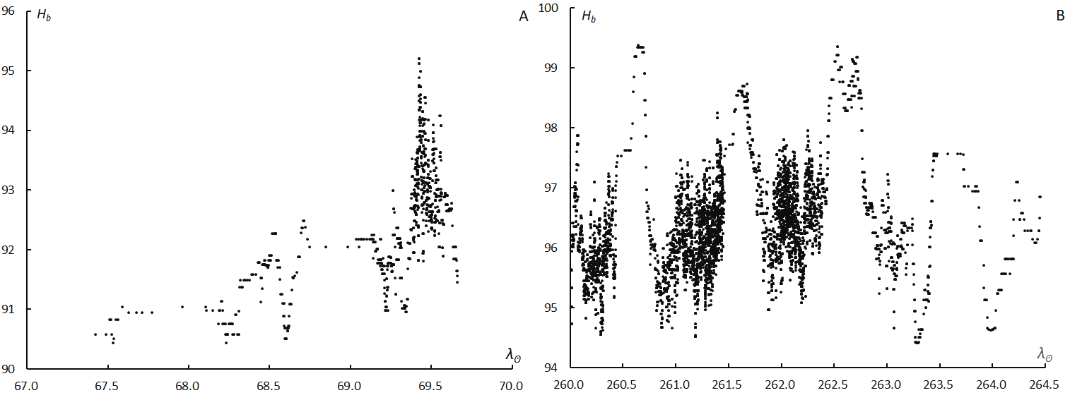
Figure 14 – Beginning height with time around the maximum. (A); τ Herculids, (B); Geminids.
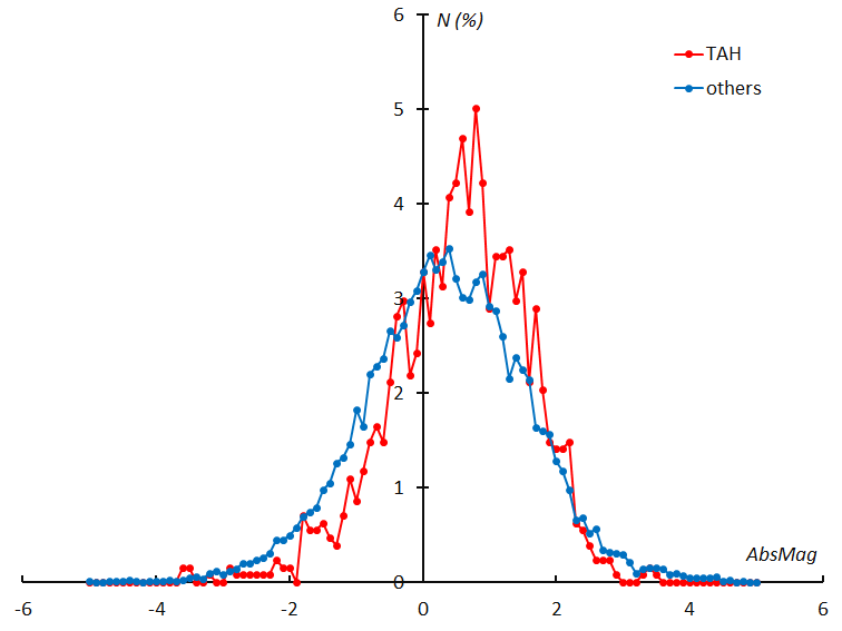
Figure 15 – Frequency distribution of the absolute magnitude of the τ Herculids compared to the distribution of other meteors that appeared during the survey (63° < λʘ < 73°).
3.5.4. Absolute magnitude
We realize that meteoroids of nTAH are unique and we suppose that their absolute magnitude distribution might be also unique. Figure 15 compares the frequency distributions of the nTAH with other meteors that appeared in the same time period. It is clear that the nTAH meteors are fainter than other meteors, but this does not mean meteoroids of nTAH are smaller than others. The luminous efficiency changes a lot with meteoroid velocity and the velocity of the nTAH is much lower than that of other meteors.
It is suggested that the absolute magnitude might change with the elevation as the beginning height changes. Figure 16A shows that the absolute magnitude of the nTAH decreases with the elevation in contrast to the Geminids case (Figure 16B). But we should be careful to conclude this because the absolute magnitude reaches the minimum at the maximum activity (Figure 16A). Camera operators of GMN in Western America met the activity maximum at the radiant culmination (see 3.3 Activity profile).
We observe brighter meteors around the shower maximum as in the case of Geminids (Figure 17B). The minimum of the absolute magnitude occurs just after the activity maximum in the Geminids but just at the activity maximum in the case of the nTAH (Figure 17A). nTAH meteoroids are so unique that both the beginning height and the absolute magnitude reach their extremes at the activity maximum (λʘ = 69.4°). Cook (1973) estimated ‘Class C’ as the residue of the surface of a cometary nucleus, that is, very porous and fragile particles. The meteoroids at the maximum of the nTAH can be considered as the most porous and fragile. Hawkins and Southworth give the following formula (Hawkins and Southworth, 1958). The intensity of light is inversely proportional to the 2/3 power of the density of the meteoroid. It is clear that the meteoroids at the nTAH maximum are more porous than those of the outskirts.
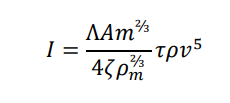
Where I is the intensity of light, is the efficiency of the energy exchange, A is the shape factor, m and ρm are the mass and the density of the meteoroid, ζ is the energy required to ablate one gram of the meteoroid, τ is the fraction of the kinetic energy converted into light, ρ is the density of the atmosphere, v is the velocity of the meteoroid.
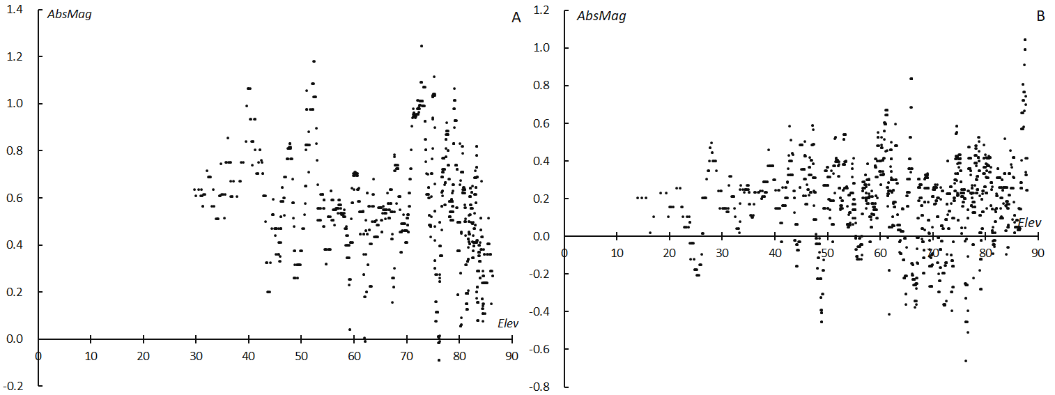
Figure 16 – Absolute magnitude and elevation angle. (A); τ Herculids, (B); Geminids.
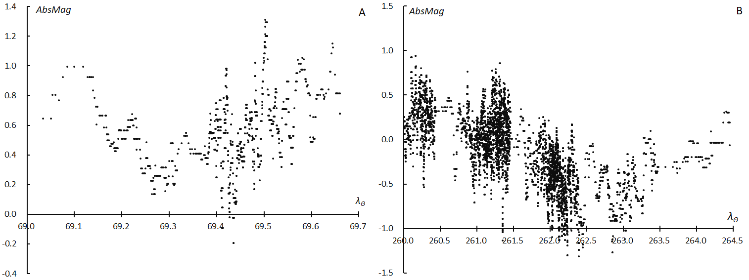
Figure 17 – Absolute magnitude with time around the maximum. (A); τ Herculids, (B); Geminids.
3.6 Extent of meteoroid stream
We realize that the elongated shape of the nTAH radiant distribution is peculiar (Figure 4A~C). Figure 18 shows the perihelion distribution corresponding to the radiant distribution of Figure 4B (69.0° < λʘ < 69.5°). It is clear the radiant distribution is caused by nTAH meteoroids distributed along with the orbital plane of the comet 73P/Schwassmann-Wachmann3. We witnessed a meteor shower of a newly formed meteoroid stream which has not yet dispersed widely.
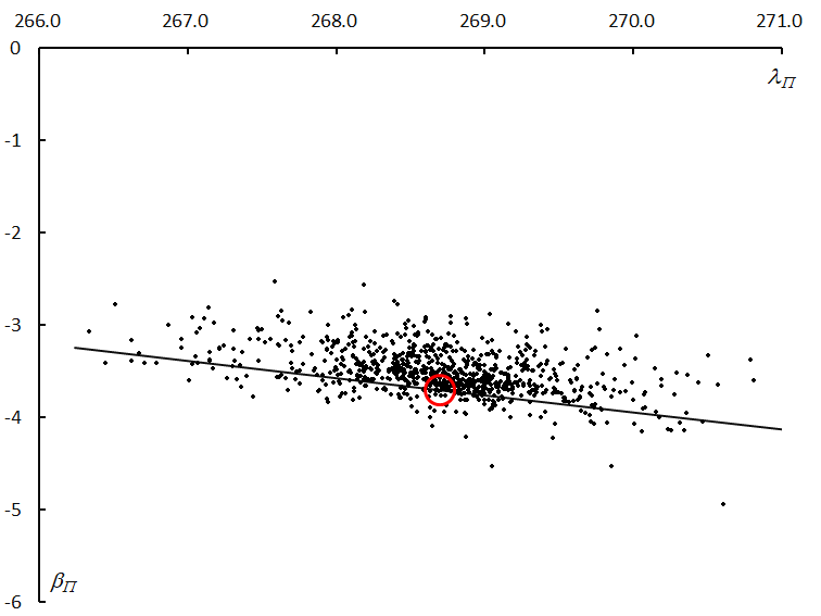
Figure 18 – Perihelion distribution of the τ Herculid meteoroids corresponding to Figure 4B (69.0° < λʘ < 69.5°). The black line shows the orbital plane of 73P/Schwassmann-Wachmann3 and the red circle indicates the position at its perihelion.
It seems to be appropriate that we do not call this meteor shower outburst of 2022 by the name of the τ Herculids (TAH). It is better to call this shower the 73P/Schwassmann-Wachmann 3ids or SW3ids; suffix -ids means ‘descendants of’ or ‘children of’. This shower does not represent the children of Hercules.
Acknowledgment
We appreciate the daily efforts by all camera operators of the Global Meteor Network. This analysis owes to their work. If GMN would be a bit idle and publish data too slowly, we would not reach the important view for this invaluable event.
This analysis relied upon the publicly available data from the GMN group under license (Vida et al., 2019; 2020; 2021).
References
Ceplecha Z. (1968). “Discrete Levels of Meteor Beginning Height”. Smithsonian Astrophysical Observatory Special Report, 279, 54 pages.
Cook A. F. (1973). “Discrete Levels of Beginning Height of Meteors in Streams”. Smithsonian Contributions to Astrophysics, 14, 1–10.
Hawkins G. S. and Southworth R. B. (1958). “The statistics of meteors in the Earth’s atmosphere”. Smithsonian Contributions to Astrophysics, 2, 349–364.
Komaki K. (1935). “On the meteoric shower associated with comet 1930VI (Schwassmann-Wachmann)”. Astronomische Nachrichten, 256, 233–234.
Koseki M. (1982). “Meteor Shower Research on Photographic Meteors by Cluster analysis”. 23rd Japanese Meteor Conference. (In Japanese).
Lindblad B. A. (1971). “A Computerized Stream Search among 2401 Photographic Meteor Orbits”. Smithsonian Contributions to Astrophysics, 12,
14–24.
Nakamura K. (1930). “On the Observation of Faint Meteors, as experienced in the case of those from the ‘Orbit of Comet Schwassmann-Wachmann, 1930c”. Monthly Notices of the Royal Astronomical Society, 91, 204–209.
SonotaCo (2009). “A meteor shower catalog based on video observations in 2007–2008”. WGN, Journal of the IMO, 37, 55–62.
Southworth R. B. and Hawkins G. S. (1963). “Statistics of meteor streams”. Smithsonian Contributions to Astrophysics, 7, 261–285.
Vida D., Gural P., Brown P., Campbell-Brown M., Wiegert P. (2019). “Estimating trajectories of meteors: an observational Monte Carlo approach – I. Theory”. Monthly Notices of the Royal Astronomical Society, 491, 2688–2705.
Vida D., Gural P., Brown P., Campbell-Brown M., Wiegert P. (2020). “Estimating trajectories of meteors: an observational Monte Carlo approach – II. Results”. Monthly Notices of the Royal Astronomical Society, 491, 3996–4011.
Vida D., Šegon D., Gural P. S., Brown P. G., McIntyre M. J. M., Dijkema T. J., Pavletić L., Kukić P., Mazur M. J., Eschman P., Roggemans P., Merlak A., Zubrović D. (2021). “The Global Meteor Network – Methodology and first results”. Monthly Notices of the Royal Astronomical Society, 506, 5046–5074.
Appendix
Estimated elements of TAH resulting from the regression analysis.
| λʘ (°) |
λ – λʘ (°) |
β (°) |
α (°) |
δ (°) |
vg (km/s) |
e | q (AU) |
i (°) |
ω (°) |
Ω (°) |
λΠ (°) |
βΠ (°) |
a (AU) |
| 65 | 128.8 | 12.6 | 197.6 | 6.1 | 9.8 | 0.607 | 0.982 | 3.3 | 203.3 | 65 | 268.2 | –1.3 | 2.5 |
| 66 | 128.1 | 18 | 200 | 11 | 10.2 | 0.624 | 0.983 | 4.9 | 202.6 | 66 | 268.6 | –1.9 | 2.62 |
| 67 | 127.3 | 23.5 | 202.4 | 15.9 | 10.5 | 0.636 | 0.985 | 6.4 | 201.9 | 67 | 268.8 | –2.4 | 2.71 |
| 68 | 126.5 | 28.9 | 204.9 | 20.8 | 10.9 | 0.643 | 0.987 | 8.1 | 201 | 68 | 268.8 | –2.9 | 2.76 |
| 69 | 125.7 | 34.3 | 207.5 | 25.7 | 11.2 | 0.643 | 0.99 | 9.7 | 200 | 69 | 268.7 | –3.3 | 2.77 |
| 69.1 | 125.6 | 34.9 | 207.8 | 26.2 | 11.3 | 0.643 | 0.99 | 9.9 | 199.9 | 69.1 | 268.7 | –3.3 | 2.77 |
| 69.2 | 125.5 | 35.4 | 208 | 26.7 | 11.3 | 0.642 | 0.99 | 10.1 | 199.7 | 69.2 | 268.7 | –3.4 | 2.77 |
| 69.3 | 125.4 | 36 | 208.3 | 27.2 | 11.3 | 0.642 | 0.991 | 10.2 | 199.6 | 69.3 | 268.6 | –3.4 | 2.77 |
| 69.4 | 125.3 | 36.5 | 208.6 | 27.7 | 11.4 | 0.642 | 0.991 | 10.4 | 199.5 | 69.4 | 268.6 | –3.5 | 2.77 |
| 69.5 | 125.2 | 37 | 208.8 | 28.2 | 11.4 | 0.641 | 0.991 | 10.6 | 199.4 | 69.5 | 268.6 | –3.5 | 2.76 |
| 69.6 | 125.1 | 37.6 | 209.1 | 28.7 | 11.4 | 0.641 | 0.992 | 10.7 | 199.3 | 69.6 | 268.6 | –3.5 | 2.76 |
| 69.7 | 125 | 38.1 | 209.4 | 29.2 | 11.5 | 0.64 | 0.992 | 10.9 | 199.2 | 69.7 | 268.5 | –3.6 | 2.75 |
| 69.8 | 124.9 | 38.7 | 209.7 | 29.6 | 11.5 | 0.639 | 0.992 | 11.1 | 199 | 69.8 | 268.5 | –3.6 | 2.75 |
| 69.9 | 124.8 | 39.2 | 209.9 | 30.1 | 11.5 | 0.638 | 0.993 | 11.2 | 198.9 | 69.9 | 268.5 | –3.6 | 2.75 |
| 70 | 124.7 | 39.8 | 210.2 | 30.6 | 11.6 | 0.638 | 0.993 | 11.4 | 198.8 | 70 | 268.4 | –3.7 | 2.74 |
| 71 | 123.5 | 45.2 | 213.1 | 35.5 | 11.9 | 0.626 | 0.996 | 13.1 | 197.4 | 71 | 268 | –3.9 | 2.66 |
| 72 | 122.1 | 50.6 | 216.1 | 40.3 | 12.3 | 0.608 | 1 | 14.8 | 195.8 | 72 | 267.3 | –4 | 2.55 |
| 73 | 120.4 | 56 | 219.5 | 45.2 | 12.7 | 0.583 | 1.003 | 16.5 | 194 | 73 | 266.4 | –3.9 | 2.41 |
| 74 | 118.1 | 61.3 | 223.2 | 49.9 | 13 | 0.552 | 1.007 | 18.1 | 191.8 | 74 | 265.2 | –3.7 | 2.25 |
| 75 | 114.8 | 66.6 | 227.5 | 54.6 | 13.4 | 0.515 | 1.01 | 19.8 | 189.2 | 75 | 263.7 | –3.1 | 2.08 |