The April Lyrids (LYR#006)

By Paul Roggemans, Carl Johannink and Koen Miskotte

A case study is presented on the April Lyrid meteor shower, based on 23083 orbits observed between solar longitude 20° and 45°. A reference orbit was derived by an iterative procedure resulting in 3220 Lyrid orbits that fulfil the low threshold D-criteria. The orbit concentration is very dense near the stream maximum with a compact radiant with more dispersed orbits at the edges of the activity period. The radiant drift was compared for different threshold classes of D-criteria. An activity profile was obtained, and the time of maximum was found to be at solar longitude 32.18 ± 0.05° instead of 32.3°. The stream shows a remarkable spread in inclination and geocentric velocities.

 

1 Introduction

The weather has been very favorable to observe the 2018 Lyrids by the CAMS BeNeLux network (Johannink and Roggemans, 2018) as well as by visual observers (Miskotte, 2018a, 2018b). The video results included 106 Lyrid orbits which fitted the high threshold criteria with D_D < 0.04 and these were used to calculate the Lyrid radiant drift. The results differed slightly from earlier results and also from an independent analysis on EDMOND and SonotaCo data.

The visual observations were used to investigate the activity profile and an attempt was made to pinpoint the time of maximum activity. The time of maximum activity differs from literature values, mainly due to a lack of visual data for several time bins.

With many Lyrid orbits available in public datasets it may be possible to consider these aspects more in detail and perhaps find an explanation for the differences between the 2018 and earlier results?

 

2 The available Lyrid orbit data

We have the following orbit data collected over 11 years, status as until July 2018, available for our search:

• EDMOND EU+world with 317830 orbits (until 2016). EDMOND collects data from different European networks which altogether operate 311 cameras (Kornos et al., 2014).
• SonotaCo with 257010 orbits (2007–2017). SonotaCo is an amateur video network with over 100 cameras in Japan (SonotaCo, 2009).
• CAMS with 111233 orbits (October 2010 – March 2013), (Jenniskens et al., 2011). For clarity, the CAMS BeNeLux orbits April 2013 – July 2018 are not included in this dataset because this data is still under embargo.

The methodology to detect associated orbits has been explained in previous analyses (Roggemans and Johannink, 2018; Roggemans, 2018; Roggemans and Campbell-Burns, 2018a, 2018b, 2018c, 2018d and 2018e). First of all the outer limits within which Lyrid orbits may be detected were obtained as follows:

• Time interval: 20° < λ_ʘ < 45°;
• Radiant area: 259° < α < 286° & +25° < δ < +43°;
• Velocity: 40 km/s < v_g < 52 km/s.

In total 23083 orbits were available in the considered time interval; 3953 orbits had a radiant position and geocentric velocity within the range mentioned above.

The D-criteria used are these of Southworth and Hawkins (1963), Drummond (1981) and Jopek (1993). We consider five different threshold levels of similarity:

• Low: D_SH < 0.25 & D_D < 0.105 & D_H < 0.25;
• Medium low: D_SH < 0.2 & D_D < 0.08 & D_H < 0.2;
• Medium high: D_SH < 0.15 & D_D < 0.06 & D_H < 0.15;
• High: D_SH < 0.1 & D_D < 0.04 & D_H < 0.1.
• Very high: D_SH < 0.05 & D_D < 0.02 & D_H < 0.05.

The purpose of this case study is to compare results with the previously published results for CAMS. For this reason, the ‘average’ orbit of the stream is obtained in the same way as by Jenniskens et al. (2016), using an ordinary median value for each orbital element. The semi-major axis a and the eccentricity e are ignored in case of hyperbolic orbits. A reference orbit for the Lyrids was derived from the selection and a few sub datasets were generated for each class of threshold level as well as for the different sources of data. The results are compared in Table 1 and Table 2. The results for the different datasets compare very well, except for the semi major axis a. The semi major axis is very sensitive for the measurement errors on velocity. The scatter on the semi major axis a for the individual orbits is very large and therefore these median values are not relevant. Both CAMS and UFOCapture are limited in accuracy to obtain the velocity of meteors, something that remains a challenge for even the most accurate observing techniques.

Table 1 – The median values for each sub-set of orbits that fulfill D_D<0.105, CAMS, SonotaCo and EDMOND and all combined orbits. The orbit from the literature is taken from Jenniskens et al. (2016).

	All	CAMS	SonotaCo	Edmond	Literature
λʘ	32.3°	32.3°	32.5°	32.2°	32.0°
αg	272.1°	272.1°	272.5°	272.0°	272.0°
δg	+33.4°	+33.4°	+33.3°	+33.4°	+33.4°
vg	46.4	46.7	46.7	46.2	46.7
a	12.5	14.0	15.5	11.4	10.8
q	0.920	0.921	0.921	0.918	0.921
e	0.938	0.953	0.952	0.928	0.956
ω	214.5°	214.0°	214.0°	214.8°	214.0°
Ω	32.3°	32.3°	32.5°	32.2°	32.3°
i	79.2°	79.4°	79.5°	79.0°	79.4°
N	3220	256	870	2094	258

 

Table 2 – The median values for the final selections of orbits for the five different threshold levels on the D-criteria.

	Low	Medium low	Medium high	High	Very high
λʘ	32.3°	32.3°	32.3°	32.3°	32.3°
αg	272.1°	272.1°	272.1°	272.1°	272.1°
δg	+33.4°	+33.4°	+33.4°	+33.4°	+33.4°
vg	46.4	46.4	46.4	46.5	46.4
a	12.5	13.2	13.9	15.5	15.1
q	0.920	0.920	0.919	0.919	0.919
e	0.938	0.940	0.941	0.942	0.939
ω	214.5°	214.5°	214.5°	214.5°	214.6°
Ω	32.3°	32.3°	32.3°	32.3°	32.3°
i	79.2°	79.2°	79.3°	79.3°	79.3°
N	3220	2890	2525	1892	803
%	81%	73%	64%	48%	22%

 

The results in Tables 1 and 2 can be compared with the orbital elements of the parent comet C/1861 G1 (Thatcher) (Jenniskens et al., 2016):

• a = 55.7 AU
• q = 0.923 AU
• e = 0.984
• ω = 213.5°
• Ω = 31.9°
• i = 79.8°

The Lyrids are considered as a major annual shower, there is no doubt about its existence. Looking at the plot of inclination versus length of perihelion, the dense concentration of orbits is obvious with a gradual spreading away from the core of the stream with very high threshold orbits towards medium low and low threshold cases dispersed at the edges of the stream (Figure 1).

 

 

About 19%, or 733 orbits of all 3953 Lyrid resembling orbits fail to fulfil the similarity criteria. Indeed, sporadic radiants are distributed all over the sky, also within the known meteor shower radiant areas. In Figure 2 we plot these 733 sporadic radiants to make the sporadic background visible which is hidden behind the color-coded Lyrid radiants shown in Figure 1. Some concentration appears at the Lyrid position in the sporadic background which is likely due to Lyrids that failed in the similarity criteria due to inaccuracies, mainly the velocity registration.

 

 

The Lyrid orbits display a large spread in orbital inclination. Figure 3 shows a close up of Figure 1 for all 3220 Lyrids with a color gradient to indicate the variation in velocity. The higher the inclination, the higher the geocentric velocity.

 

 

When we plot the geocentric velocity v_g versus inclination i for all 3220 Lyrid orbits the geocentric velocity v_g increases with 0.485 km/s per degree in inclination (Figure 4). This variation in velocity in function of the inclination is very well visible in Figure 3.

 

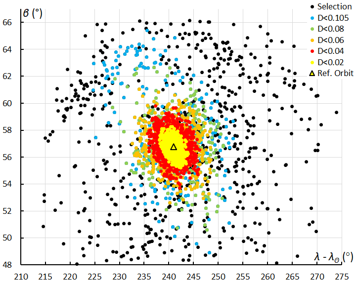
Kresák and Porubčan (1970) made a study about the dispersion of meteor orbits and the size of the radiants. For the Lyrids they found a rather small radiant area, but based on 7 Lyrid orbits only, which is too few to be statistically relevant. The dense concentration of orbits also appears in the 3220 radiant positions of this analysis, plotted in Sun centered ecliptic coordinates. The radiant is very concentrated for very high, high and medium high threshold orbits (Figure 5).

Kresák and Porubčan also calculated the variation of the orbital elements, e, q, i and ω in function of Ω. For instance, for the Lyrids they found di/dΩ = +0.24, we find +0.25. However, the scatter on the data points requires great caution and for this reason we do not go into further detail on this point.

 

 

 

 

We also show the plot of the ecliptic latitude β against the Sun centered longitude λ – λ_ʘ for the 733 sporadic orbits of the 3953 selected orbits (Figure 6). Mind that any single station observing method has no possibility to distinguish these sporadics from Lyrids! In Figure 7 we see the 3220 Lyrid radiants with the variation in velocity. From Figure 3 we know that the higher the velocity, the higher the inclination, hence the lower inclination Lyrid orbits are in the upper left corner, the higher inclination orbits in the bottom right corner of Figure 7.

Plotting the geocentric velocity v_g against the solar longitude, the velocity increases with 0.11 km/s per degree in solar longitude. Earth travers the Lyrid stream from the inner to the outer side, encountering first slower Lyrids and gradually slightly faster Lyrids.

The Lyrids do not display high hourly rates, unless in certain years when outbursts surprised observers. With its in general rather low hourly rates this shower is an interesting case to compare with the so-called minor showers, some of which reach comparable activity levels. Note that in Table 2 as many as 81% of all possible Lyrids fulfil the low threshold D-Criteria. The Lyrids presence in the selected dataset is very distinct, something that makes the difference with most minor showers.

 

3 Radiant drift

The CAMS BeNeLux results of 2018 were used to derive the radiant drift (Johannink and Roggemans, 2018). The results differed slightly from past CAMS orbit data as well as from what was derived from past EDMOND and SonotaCo orbit data. The question arises why the results differ and how relevant the differences in resulting radiant drift really are. We therefore repeat the analysis using the Lyrid orbit selection in this case study and we do this for each of the D-criteria threshold classes.

Figures 8 and 9 display the Right Ascension and declination in function of time (solar longitude) for all different threshold classes of D-criteria. The slope of the linear regression through the datapoints is a good measure for the daily movement, or drift, of the radiant through the sky. The radiant drift is the result of the rotation of the Earth around the Sun relative to the orbit of the meteor stream and thus the direction from where the meteoroids enter the atmosphere.

When applying linear regression, the dispersion on the data points determines the relevance of the trend line. Linear regression makes no sense neither on too few datapoints, nor on a too short range. In our case Figure 8 visualizes the number, the range and the spread of the datapoints for the drift in Right Ascension. The higher the threshold level, the closer we get to the core of the meteor stream, the smaller the range becomes. From a calculation point of view the low threshold points (blue) cover the largest range in solar longitude and provide the best linear regression. However, the low threshold datapoints represent the more dispersed orbits with the poorest association to the shower.

 

 

 

Table 3 – Radiant drift with ± σ for the Lyrids obtained from the orbits for each threshold level of the D-criteria and from the 2018 study (Johannink and Roggemans, 2018 (*)).

Threshold/source	LYR – 006
	Δα / λʘ	Δδ / λʘ
Low	0.75 ± 0.02	–0.11 ± 0.02
Medium low	0.78 ± 0.02	–0.14 ± 0.02
Medium high	0.90 ± 0.03	–0.22 ± 0.02
High	1.04 ± 0.03	–0.21 ± 0.02
Very high	1.03 ± 0.04	–0.12 ± 0.03
Edmond&SonotaCo (*)	1.04 ± 0.03	–0.21 ± 0.02
Jenniskens et al. (2018)	0.66	+0.02
BeNeLux 2018 (*)	0.87 ± 0.08	–0.10 ± 0.11

 

Figure 9 shows a large spread in datapoints which is somehow problematic for a linear regression. If the datapoints would be equally distributed in x– and y– coordinates, the resulting trendline becomes meaningless. It is rather difficult to see any trend in the points in Figure 9 especially for the high and very high threshold orbits. The larger the spread on a cloud of points, the larger the uncertainty on the resulting trendline. Altogether the differences found for the radiant drift based on the different classes of threshold levels and the results found by Johannink and Roggemans (2018) listed in Table 3 are normal because of the scatter on the radiant positions. In principle radiant drift is just the resultant of the movement of the Earth and the direction of the shower orbit. The scatter on the orbits due to measurement errors and the physical dispersion of particles explain the differences in radiant drifts between different analyzes. A standard deviation on the linear regression is not representative for the error margin due to the dispersion of the orbits.

One way to verify the effect of the differences in radiant drift is to just apply these radiant drift corrections to see to which extend the resulting pictures differ. Figure 10 displays the uncorrected radiant positions for all 3953 orbits in the sample. The Lyrid radiant appears already very compact in this plot of uncorrected radiant position.

 

 

We apply the radiant drift correction with Δα/Δλ_ʘ = +0.9° and Δδ/Δλ_ʘ = –0.22°, valid for the medium high threshold orbits in this analysis (Table 3, Figure 11). We do the same with Δα/Δλ_ʘ = +0.78° and Δδ/Δλ_ʘ = –0.14°, valid for the medium low threshold orbits in this analysis (Table 3, Figure 12), and Δα/Δλ_ʘ = +0.66° and Δδ/Δλ_ʘ = +0.02° according to Jenniskens et al. (2018) (Table 3, Figure 13).

In all three cases we see that the sporadic (black) radiant points get more dispersed as the radiant drift is not valid for these meteors. The radiants of the orbits that fit the D-criteria get more concentrated in a compact radiant, showing the validity of the radiant drift correction for these radiants. Many radiants of the low threshold orbits remain with a rather large dispersion which may indicate that the radiant drift is not valid for these radiants which may be sporadics. Therefore, in some cases it is recommended not to use the low threshold class radiants for radiant drift determination. In our case, all values listed in Table 3 can be considered as a good approach of the theoretical radiant drift.

 

 

4 The activity profile and maximum

The orbit sample has been collected over 11 years from 2007 until 2017. There is no indication for any outburst in these years. The percentage of Lyrid orbits compared to the non-Lyrid orbits remains stable, ~16.2% when we consider the entire Lyrid activity interval. In the period when mainly medium high threshold orbits or better are recorded (27° < λ_ʘ < 37°) the number of Lyrid orbits reach one third (34.4%) of the number of non-Lyrid orbits. Also, the interval with the best Lyrid rates, 31.85° < λ_ʘ < 33°, appears very stable in strength from year to year. At the maximum the number of Lyrid orbits are 1.6 times (156.1%) the number of non-Lyrid orbits. The different relative activity levels are displayed in Figure 14.

 

 

The number of shower meteors per hour depends on the elevation of the radiant, the size of the unobstructed field of view and the limiting magnitude of the sky. The standard procedure for visual observers requires these data in order to calculate the Zenithal Hourly Rate or ZHR which should allow to compare the activity for observations done under different circumstances. With our orbit data we have only a total number of orbits obtained by cameras with different fields of view and different limiting magnitudes with the radiant at different elevations, no way to correct for any of these factors. With data collected over a wide range of radiant elevations, the influence on the total number of orbits per unit of time is likely to be averaged out. Video observations are much less sensitive to influences of moonlight and light pollution than visual observations. Moreover, these and other influences on the number of orbits per unit of time can be eliminated by comparing the proportion of shower orbits to the total number of non-shower orbits as the weather circumstances will affect both in the same manner. This way we can reconstruct an activity profile as a percentage of the shower orbits relative to the background activity or the total number of the remaining non-shower orbits collected in the same time interval. Figure 15 shows the activity profile obtained from the number of orbits. The profile is the same for each threshold level.

 

 

The activity is made up of mainly medium high and higher threshold level orbits. The low threshold orbits (blue) which represent outliers or perhaps sporadics that just fit the similarity criteria by pure chance, do not have any significant effect on the total activity level (Figure 15).

Koen Miskotte (2018), made an analysis of the Lyrid 2018 activity based on the available visual observations worldwide. Unfortunately, visual observing has been sadly neglected in recent years and the observational data is rather limited to Europe and few observers based in America. The theoretical maximum was not covered by observers and only some limited time spans got documented with ZHR values. To compare the 2018 ZHRs with our orbits-based activity profile we take one point from Koen Miskotte’s ZHR profile and the relative activity at the very same instance on our activity profile to calibrate all ZHR values to the relative activity level. The datapoints for these ZHR values are shown in Figure 16 and the corresponding times for the ZHR data are marked with A, B, C, D, E, F and G in Figures 16 and 17. The activity level of the visual ZHR at point ‘A’ is close to 40%, while ‘B’ is between 60% and 80%, the increase in activity is comparable in both curves, but the visual observations seem to identify more meteors as Lyrids than what we get from the orbit data.

The activity profile in Figure 17 shows a shoulder in activity between ‘B’ and ‘C’ that lasts for about 0.8 days, ending with a dip. It is at this dip that Koen has another few hours of visual data available, marked with ‘C’. Both the orbit data and the visual ZHR are close to 60%. It is not clear how to explain the scatter in ZHR values within this short interval of time. This may be due to too few observers or perhaps to some under correction of the ZHR.

From about λ_ʘ = 31.7° the Lyrid activity increases rapidly towards its maximum and half way this steep increase, Koen has another ZHR result at ‘D’. When the next time span with ZHRs is available at ‘E’, the Lyrid maximum was already over. Rendtel (2017) situates the Lyrid maximum between 32° and 32.45° in solar longitude with the time of maximum activity at λ_ʘ = 32.32° (red arrows in Figure 17 activity period marked with 1–2, the maximum with 3). The activity profile obtained from the orbit data suggest the maximum to be rather about at λ_ʘ = 32.20°.

 

 

The orbit-based activity profile does not include any 2018 data and there is no reason to assume the Lyrid activity could not have displayed short-lived fluctuations in 2018. However, the ZHRs at points ‘D’ and ‘E’ look somehow underestimated. The scatter on the ZHRs at ‘E’ is remarkable and it might be worthwhile to check if these ZHR values could have been under corrected somehow. The ZHR values at ‘F’ compares well to the orbit data, while the ZHR at ‘G’ is more than twice what we expect from the orbit data. Since the 2018 visual data is based on a fractional coverage of the Lyrid activity, it would be interesting to combine data from different years into a single ZHR profile.

Looking at Figure 17 we see that Lyrids display the best of their activity in about a week of time. Zooming in on the peak activity period, we see a shoulder (‘B’ to ‘C’) about a day ahead of the shower maximum. The main peak is skew, increasing steep from ‘C’ to the maximum, decreasing more slowly towards ‘E’, like a shoulder is imbedded on the profile. About 16 hours after the maximum another sub maximum appears on the activity profile (few hours after position ‘E’) and a final ‘shoulder’ is visible just before ‘F’. Such sub maxima, often merged in the activity profile as a ‘shoulder’, are produced by dust filaments that precede or follow the main core of the stream. Such features are typical for a layered dust distribution produced by the dynamic evolution of particles injected by the parent body at different revolutions and undergoing effects of planetary perturbations.

Based on the relative activity profile derived from the numbers of orbits collected on a global scale over 11 years of time, we can pinpoint the time of maximum at λ_ʘ = 32.18 ± 0.05°, while λ_ʘ = 32.3° is in fact the median value of the entire activity period. The different characteristics of the orbit-based activity profile are present in all classes of threshold of D-criteria and therefore pretty sure not just spurious effects.

 

5 Other shower characteristics

With a geocentric velocity of 46.4 km/s the Lyrids produce a luminous trajectory in the atmospheric layer between 105 and 90 km elevation. This is between the higher layer where fast meteors such as Leonids, Orionids or Perseids appear, and the lower level where slow meteors such as Taurids, Draconids, etc can be expected. This layer is very well covered by all camera networks optimized for 90 kilometers or lower.

 

Table 4 – Beginning and ending heights with ± σ for the Lyrids obtained from the trajectories for each threshold level of the D-criteria.

Threshold level	LYR – 006
	Hbeg	Hend
Low	104.8 ± 4.3 km	90.3 ± 6.3 km
Medium low	104.8 ± 4.2 km	90.2 ± 6.3 km
Medium high	104.9 ± 4.2 km	89.9 ± 6.3 km
High	105.0 ± 4.1 km	89.8 ± 6.3 km
Very high	105.2 ± 4.0 km	89.5 ± 6.1 km

 

Looking at the median values for the beginning and ending points for each class of threshold level in D-criteria, all results are in a very good agreement (Table 4). We assume that the data providers, CAMS, EDMOND and SonotaCo, list the values obtained from triangulations that represent the real begin, and ending heights. Anyway, by using median values any outliers have little or no influence.

 

Most orbits in this case study were obtained by the EDMOND and SonotaCo networks which use wide field of view optics and less sensitive cameras with a limiting magnitude for meteors of about +2.0. The CAMS networks use small field of view optics and mostly Watec H2 Ultimates, capturing meteors of up to magnitude +4.5. This explains why most orbits were obtained for relative bright meteors, compared to the range in brightness typically covered by a visual observer or by the CAMS video system. The magnitude range covered by CAMS data and the range covered by EDMOND and SonotaCo data is too different to just combine the data for further analyzes.

It might be tending to derive the population index from the the trend line through the linear segment of the histogram in Figure 18 and perhaps look at different time bins to determine possible variation of the population index. However, the suitable range is limited to –4.0 to –0.5, which cannot be straightforward compared to values from classical visual observation which mostly cover a range of –4.0 to +5.0. Another concern is that the composition of the sample based upon data from a very diverse kind of optics may be unsuitable to derive population indices. This requires a more thorough evaluation of the use of the magnitude data obtained from such variety of video optics.

Although the Lyrids produce some nice numbers of bright meteors, exceptional bright Lyrid fireballs are missing, and the magnitude distribution is less abundant in bright meteors than for instance the ζ-Cassiopeiids (Roggemans and Cambell-Burns, 2018e). The Lyrids have a Long Periodic Comet type orbit and are associated with Comet C/1861 G1 (Thatcher) which moves in an orbit with a periodicity of about 415 years. This may be the reason why the smaller particles were better preserved and why the proportion bright Lyrids is less abundant than for other orbit types. Our sample of 3220 Lyrid orbits had an average absolute magnitude, brightest and faintest value of –1.1 [–7.2; +2.6]. The magnitude distribution as a percentage of the total number of Lyrids is shown in Figure 18.

If we calculate the average absolute magnitude for each interval of 0.5° in solar longitude with a step of 0.25° solar longitude for all 19840 non-Lyrid meteors in the considered period and for all 3220 Lyrid orbits, we see that the Lyrids are about 1 magnitude brighter than the overall meteor activity (Figure 19). The graph shows a trend that indicates the average Lyrid magnitude becomes brighter throughout the activity period. This could indicate some mass sorting meaning that Earth enters the Lyrid stream where it is richer in small particles and gradually encounters proportional more larger particles. This should be visible in an analyzes of visual observations as a decreasing value for the population index.

However, the geocentric velocity v_g shows a trend in function of the solar longitude λ_ʘ, with slight slower speeds than the average when Earth enters the Lyrid stream, gradually increasing during the transit of the Earth through the stream. We see this velocity distribution very distinctly in the radiant plot (Figure 7) as well as in the plot of inclination i against the length of perihelion Π (Figure 3). The increase in brightness during the Lyrid activity can be partially explained by the increase in velocity as the faster a particle with a given mass moves, the more energy it has and the brighter the meteor will be. With an increase of 0.11 km/s per degree in solar longitude, the increase in velocity over the 9° in solar longitude as shown in Figure 19 cannot explain the increase of 0.6 magnitude. The most likely explanation is some particle size sorting with the smaller particles being encountered first as these got towards the inner side of the stream due to the Poynting-Robertson drag. More research remains to be done to assess to which extent the increasing velocity accounts for the increase in brightness and how much is due to the particle size sorting. If the mass sorting effect can be estimated, it might be possible to get an idea of the age of the stream as how much time was needed to get at the current stage of mass sorting.

 

 

 

6 Conclusion

In this case study the authors found that the differences in radiant drift in the 2018 Lyrid analyzes which puzzled the authors, are not a problem, all values are a good approach of the resultant of the movement of Earth and the direction of the shower orbit, within the uncertainty limits for the method to obtain the radiant drift. The statistical standard deviation which is found for the slope of the linear regression is rather small due to the large number of data points but not representative for the physical properties of the sample, including the error margins on the data points.

The ZHR curve for the 2018 Lyrids was very fragmentary due to a lack of global coverage. Converting the visual ZHR values to a percentage as a relative activity level allows to compare with the activity profile derived from the percentage of shower orbits per unit of time relative to the number of non-shower orbits. The 2018 visual observers had missed the hours with the Lyrid maximum, but the observed activity levels on different dates can be compared with the activity profile based on 11 years of orbital data. The time of maximum activity appears rather at λ_ʘ = 32.18 ± 0.05° instead of λ_ʘ = 32.3° like mentioned in literature (Rendtel, 2017).

Contrary to other major showers, Lyrids are not abundant in bright and very bright events. The Lyrid stream contains still a large portion of small particles. During the transit of the Earth through the Lyrid stream, the average velocity and the average brightness of the particles increase.

 

Acknowledgment

We thank Denis Vida for providing us with a tool to plot a color gradient to show the dispersion in velocity and for his critical reviewing of this case study.

The authors are very grateful to Jakub Koukal for updating the dataset of EDMOND with the most recent data, to SonotaCo Network (Simultaneously Observed Meteor Data Sets SNM2007–SNM2017), to CAMS (2010–2013) and to all camera operators involved in these camera networks.

EDMOND (https://fmph.uniba.sk/microsites/daa/daa/veda-a-vyskum/meteory/edmond/) includes: BOAM (Base des Observateurs Amateurs de Meteores, France), CEMeNt (Central European Meteor Network, cross-border network of Czech and Slovak amateur observers), CMN (Croatian Meteor Network or HrvatskaMeteorskaMreza, Croatia), FMA (Fachgruppe Meteorastronomie, Switzerland), HMN (HungarianMeteor Network or Magyar Hullocsillagok Egyesulet, Hungary), IMO VMN (IMO Video Meteor Network), MeteorsUA (Ukraine), IMTN (Italian amateur observers in Italian Meteor and TLE Network, Italy), NEMETODE (Network for Meteor Triangulation and Orbit Determination, United Kingdom), PFN (Polish Fireball Network or Pracownia Komet i Meteorow, PkiM, Poland), Stjerneskud (Danish all-sky fireball cameras network, Denmark), SVMN (Slovak Video Meteor Network, Slovakia), UKMON (UK Meteor Observation Network, United Kingdom).

References

Drummond J. D. (1981). “A test of comet and meteor shower associations”. Icarus, 45, 545–553.

Jenniskens P., Gural P. S., Grigsby B., Dynneson L., Koop M. and Holman D. (2011). “CAMS: Cameras for Allsky Meteor Surveillance to validate minor meteor showers”. Icarus, 216, 40–61.

Jenniskens P., Nénon Q., Albers J., Gural P. S., Haberman B., Holman D., Morales R., Grigsby B. J., Samuels D. and Johannink C. (2016). “The established meteor showers as observed by CAMS”. Icarus, 266, 331–354.

Jenniskens P., Baggaley J., Crumpton I., Aldous P., Pokorny P., Janches D., Gural P. S., Samuels D., Albers J., Howell A., Johannink C., Breukers M., Odeh M., Moskovitz N., Collison J. and Ganjuag S. (2018). “A survey of southern hemisphere meteor showers”. Planetary Space Science, 154, 21–29.

Jopek T. J. (1993). “Remarks on the meteor orbital similarity D-criterion”. Icarus, 106, 603–607.

Kornoš L., Matlovič P., Rudawska R., Tóth J., Hajduková M. Jr., Koukal J. and Piffl R. (2014). “Confirmation and characterization of IAU temporary meteor showers in EDMOND database”. In Jopek T. J., Rietmeijer F. J. M., Watanabe J., Williams I. P., editors, Proceedings of the Meteoroids 2013 Conference, Poznań, Poland, Aug. 26-30, 2013. A.M. University, pages 225–233.

Kresák L. and Porubčan V. (1970). “The dispersion of meteors in meteor streams. I. The size of the radiant areas”. Bulletin of the Astronomical Institute of Czechoslovakia, 21, 153–170.

Johannink C. and Roggemans P. (2018). “CAMS BeNeLux: results April 2018”. eMetN, 3, 192–194.

Miskotte K. (2018a). “Lyrid 2018 observations from Ermelo, the Netherlands”. eMetN, 3, 195–197.

Miskotte K. (2018b). “Lyrids 2018: an analysis”. eMetN, 3, 204–206.

Rendtel J. (2017). “2018 Meteor shower calendar”. IMO.

Roggemans P. (2018). “August gamma Cepheids (523-AGC)”. eMetN, 3, 73–78.

Roggemans P. and Cambell-Burns P. (2018a). “x Herculids (XHE-346)”. eMetN, 3, 120–127.

Roggemans P. and Cambell-Burns P. (2018b). “February Hydrids (FHY-1032)”. eMetN, 3, 128–133.

Roggemans P. and Cambell-Burns P. (2018c). “Alpha Aquariids (AAQ-927)”. eMetN, 3, 134–141.

Roggemans P. and Cambell-Burns P. (2018d). “Eta Lyrids (ELY-145)”. eMetN, 3, 142–147.

Roggemans P. and Cambell-Burns P. (2018e). “Zeta Cassiopeiids (ZCS-444)”. eMetN, 3, 225–232.

Roggemans P. and Johannink C. (2018). “A search for December alpha Bootids (497)”. eMetN, 3, 64–72.

SonotaCo (2009). “A meteor shower catalog based on video observations in 2007-2008”. WGN, Journal of the International Meteor Organization, 37, 55–62.

Southworth R. R. and Hawkins G. S. (1963). “Statistics of meteor streams”. Smithson. Contrib. Astrophys., 7, 261–286.